35 KiB
Closed-Loop Shaping using Complementary Filters
\bibliographystyle{IEEEtran}
Title Page ignore
Introduction ignore
Once the system is properly decoupled using one of the approaches described in Section ref:sec:detail_control_decoupling, SISO controllers can be individually tuned for each decoupled "directions". Several ways to design a controller to obtain a given performance while ensuring good robustness properties can be implemented.
In some cases "fixed" controller structures are utilized, such as PI and PID controllers, whose parameters are manually tuned cite:&furutani04_nanom_cuttin_machin_using_stewar;&du14_piezo_actuat_high_precis_flexib;&yang19_dynam_model_decoup_contr_flexib.
Another popular method is Open-Loop shaping, which was used during the conceptual phase. Open-loop shaping involves tuning the controller through a series of "standard" filters (leads, lags, notches, low-pass filters, …) to shape the open-loop transfer function $G(s)K(s)$ according to desired specifications, including bandwidth, gain and phase margins cite:&schmidt20_desig_high_perfor_mechat_third_revis_edition, chapt. 4.4.7. Open-Loop shaping is very popular because the open-loop transfer function is a linear function of the controller, making it relatively straightforward to tune the controller to achieve desired open-loop characteristics. Another key advantage is that controllers can be tuned directly from measured frequency response functions of the plant without requiring an explicit model.
However, the behavior (i.e. performance) of a feedback system is a function of closed-loop transfer functions. Specifications can therefore be expressed in terms of the magnitude of closed-loop transfer functions, such as the sensitivity, plant sensitivity, and complementary sensitivity transfer functions cite:&skogestad07_multiv_feedb_contr, chapt. 3. With open-loop shaping, closed-loop transfer functions are changed only indirectly, which may make it difficult to directly address the specifications that are in terms of the closed-loop transfer functions.
In order to synthesize a controller that directly shapes the closed-loop transfer functions (and therefore the performance metric), $\mathcal{H}_\infty\text{-synthesis}$ may be used cite:&skogestad07_multiv_feedb_contr. This approach requires a good model of the plant and expertise in selecting weighting functions that will define the wanted shape of different closed-loop transfer functions cite:&bibel92_guidel_h. $\mathcal{H}_{\infty}\text{-synthesis}$ has been applied for the Stewart platform cite:&jiao18_dynam_model_exper_analy_stewar, yet when benchmarked against more basic decentralized controllers, the performance gains proved small cite:&thayer02_six_axis_vibrat_isolat_system;&hauge04_sensor_contr_space_based_six.
In this section, an alternative controller synthesis scheme is proposed in which complementary filters are used for directly shaping the closed-loop transfer functions (i.e., directly addressing the closed-loop performances). In Section ref:ssec:detail_control_cf_control_arch, the proposed control architecture is presented. In Section ref:ssec:detail_control_cf_trans_perf, typical performance requirements are translated into the shape of the complementary filters. The design of the complementary filters is briefly discussed in Section ref:ssec:detail_control_cf_analytical_complementary_filters, and analytical formulas are proposed such that it is possible to change the closed-loop behavior of the system in real time. Finally, in Section ref:ssec:detail_control_cf_simulations, a numerical example is used to show how the proposed control architecture can be implemented in practice.
Control Architecture
<<ssec:detail_control_cf_control_arch>>
Virtual Sensor Fusion
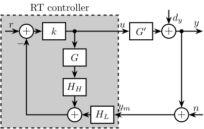
The idea of using complementary filters in the control architecture originates from sensor fusion techniques cite:&collette15_sensor_fusion_method_high_perfor, where two sensors are combined using complementary filters. Building upon this concept, "virtual sensor fusion" cite:&verma20_virtual_sensor_fusion_high_precis_contr replaces one physical sensor with a model $G$ of the plant. The corresponding control architecture is illustrated in Figure ref:fig:detail_control_cf_arch, where $G^\prime$ represents the physical plant to be controlled, $G$ is a model of the plant, $k$ is the controller, and $H_L$ and $H_H$ are complementary filters satisfying $H_L(s) + H_H(s) = 1$. In this arrangement, the physical plant is controlled at low frequencies, while the plant model is utilized at high frequencies to enhance robustness.
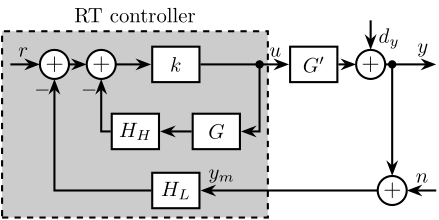
Although the control architecture shown in Figure ref:fig:detail_control_cf_arch appears to be a multi-loop system, it should be noted that no non-linear saturation-type elements are present in the inner loop (containing $k$, $G$, and $H_H$, all numerically implemented). Consequently, this structure is mathematically equivalent to the single-loop architecture illustrated in Figure ref:fig:detail_control_cf_arch_eq.
Asymptotic behavior
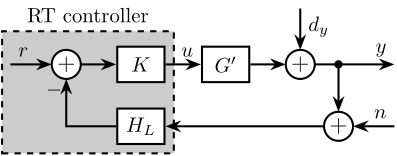
When considering the extreme case of very high values for $k$, the effective controller $K(s)$ converges to the inverse of the plant model multiplied by the inverse of the high-pass filter, as expressed in eqref:eq:detail_control_cf_high_k.
\begin{equation}\label{eq:detail_control_cf_high_k} limk→∞ K(s) = limk→∞ \frac{k}{1+H_H(s) G(s) k} = \big( H_H(s) G(s) \big)-1
\end{equation}
If the resulting $K$ is improper, a low-pass filter with sufficiently high corner frequency can be added to ensure its causal realization. Furthermore, for $K$ to be stable, both $G$ and $H_H$ must be minimum phase transfer functions.
With these assumptions, the resulting control architecture is illustrated in Figure ref:fig:detail_control_cf_arch_class, where the complementary filters $H_L$ and $H_H$ remain the only tuning parameters. The dynamics of this closed-loop system are described by equations eqref:eq:detail_control_cf_cl_system_y and eqref:eq:detail_control_cf_cl_system_y.
\begin{subequations}\label{eq:detail_control_cf_sf_cl_tf_K_inf}
\begin{align} y &= \frac{ H_H dy + G^{\prime} G^{-1} r - G^{\prime} G^{-1} H_L n }{H_H + G^\prime G^{-1} H_L} \label{eq:detail_control_cf_cl_system_y}\\ u &= \frac{ -G^{-1} H_L dy + G^{-1} r - G^{-1} H_L n }{H_H + G^\prime G^{-1} H_L} \label{eq:detail_control_cf_cl_system_u} \end{align}\end{subequations}
At frequencies where the model accurately represents the physical plant ($G^{-1} G^{\prime} \approx 1$), the denominator simplifies to $H_H + G^\prime G^{-1} H_L \approx H_H + H_L = 1$, and the closed-loop transfer functions are then described by equations eqref:eq:detail_control_cf_cl_performance_y and eqref:eq:detail_control_cf_cl_performance_u.
\begin{subequations}\label{eq:detail_control_cf_sf_cl_tf_K_inf_perfect}
\begin{alignat}{5}
y &= H_H dy &&+ r &&- H_L n \label{eq:detail_control_cf_cl_performance_y}
u &= -G-1 H_L dy &&+ G-1 r &&- G-1 H_L n \label{eq:detail_control_cf_cl_performance_u}
\end{alignat}
\end{subequations}
The sensitivity transfer function equals the high-pass filter $S = \frac{y}{dy} = H_H$, and the complementary sensitivity transfer function equals the low-pass filter $T = \frac{y}{n} = H_L$. Hence, when the plant model closely approximates the actual dynamics, the closed-loop transfer functions converge to the designed complementary filters, allowing direct translation of performance requirements into the design of the complementary.
Translating the performance requirements into the shape of the complementary filters
<<ssec:detail_control_cf_trans_perf>>
Introduction ignore
Performance specifications in a feedback system can usually be expressed as upper bounds on the magnitudes of closed-loop transfer functions such as the sensitivity and complementary sensitivity transfer functions cite:&bibel92_guidel_h. The design of a controller $K(s)$ to obtain the desired shape of these closed-loop transfer functions is known as closed-loop shaping.
In the proposed control architecture, the closed-loop transfer functions eqref:eq:detail_control_cf_sf_cl_tf_K_inf are expressed in terms of the complementary filters $H_L(s)$ and $H_H(s)$ rather than directly through the controller $K(s)$. Therefore, performance requirements must be translated into constraints on the shape of these complementary filters.
Nominal Stability (NS)
A closed-loop system is stable when all its elements (here $K$, $G^\prime$, and $H_L$) are stable and the sensitivity function $S = \frac{1}{1 + G^\prime K H_L}$ is stable. For the nominal system ($G^\prime = G$), the sensitivity transfer function equals the high-pass filter: $S(s) = H_H(s)$.
Nominal stability is therefore guaranteed when $H_L$, $H_H$, and $G$ are stable, and both $G$ and $H_H$ are minimum phase (ensuring $K$ is stable). Consequently, stable and minimum phase complementary filters must be employed.
Nominal Performance (NP)
Performance specifications can be formalized using weighting functions $w_H$ and $w_L$, where performance is achieved when eqref:eq:detail_control_cf_weights is satisfied. The weighting functions define the maximum magnitude of the closed-loop transfer functions as a function of frequency, effectively determining their "shape".
\begin{subequations}\label{eq:detail_control_cf_weights}
\begin{align} |w_H(j\omega) S(j\omega)| &\le 1 \quad \forall\omega\\ |w_L(j\omega) T(j\omega)| &\le 1 \quad \forall\omega \end{align}\end{subequations}
For the nominal system, $S = H_H$ and $T = H_L$, hence the performance specifications can be converted on the shape of the complementary filters eqref:eq:detail_control_cf_nominal_performance.
\begin{equation}\label{eq:detail_control_cf_nominal_performance} \Aboxed{\text{NP} \Longleftrightarrow {\begin{cases*}
| w_H(jω) H_H(jω) | ≤ 1 & ∀ω \\ |
| w_L(jω) H_L(jω) | ≤ 1 & ∀ω |
\end{cases*}}}
\end{equation}
For disturbance rejection, the magnitude of the sensitivity function $|S(j\omega)| = |H_H(j\omega)|$ should be minimized, particularly at low frequencies where disturbances are usually most prominent. Similarly, for noise attenuation, the magnitude of the complementary sensitivity function $|T(j\omega)| = |H_L(j\omega)|$ should be minimized, especially at high frequencies where measurement noise typically dominates. Classical stability margins (gain and phase margins) are also related to the maximum amplitude of the sensitivity transfer function. Typically, maintaining $|S|_{\infty} \le 2$ ensures a gain margin of at least 2 and a phase margin of at least $\SI{29}{\degree}$.
Therefore, by carefully selecting the shape of the complementary filters, nominal performance specifications can be directly addressed in an intuitive manner.
Robust Stability (RS)
Robust stability refers to a control system's ability to maintain stability despite discrepancies between the actual system $G^\prime$ and the model $G$ used for controller design. These discrepancies may arise from unmodeled dynamics or nonlinearities.
To represent these model-plant differences, input multiplicative uncertainty as illustrated in Figure ref:fig:detail_control_cf_input_uncertainty is employed. The set of possible plants $\Pi_i$ is described by eqref:eq:detail_control_cf_multiplicative_uncertainty, with the weighting function $w_I$ selected such that all possible plants $G^\prime$ are contained within the set $\Pi_i$.
\begin{equation}\label{eq:detail_control_cf_multiplicative_uncertainty} Π_i: \quad G^′(s) = G(s)\big(1 + w_I(s)Δ_I(s)\big); \quad |Δ_I(jω)| ≤ 1 \ ∀ω
\end{equation}
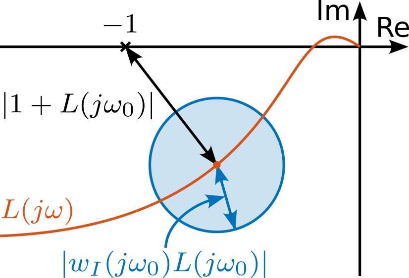
When considering input multiplicative uncertainty, robust stability can be derived graphically from the Nyquist plot (illustrated in Figure ref:fig:detail_control_cf_nyquist_uncertainty), yielding to eqref:eq:detail_control_cf_robust_stability_graphically, as demonstrated in cite:&skogestad07_multiv_feedb_contr, chapt. 7.5.1.
\begin{equation}\label{eq:detail_control_cf_robust_stability_graphically} \text{RS} \Longleftrightarrow ≤ft|w_I(jω) L(jω) \right| ≤ ≤ft| 1 + L(jω) \right| \quad ∀ω
\end{equation}
After algebraic manipulation, robust stability is guaranteed when the low-pass complementary filter $H_L$ satisfies eqref:eq:detail_control_cf_condition_robust_stability.
\begin{equation}\label{eq:detail_control_cf_condition_robust_stability} \boxed{\text{RS} \Longleftrightarrow |w_I(jω) H_L(jω)| ≤ 1 \quad ∀ ω}
\end{equation}
Robust Performance (RP)
Robust performance ensures that performance specifications eqref:eq:detail_control_cf_weights are met even when the plant dynamics fluctuates within specified bounds eqref:eq:detail_control_cf_robust_perf_S.
\begin{equation}\label{eq:detail_control_cf_robust_perf_S} \text{RP} \Longleftrightarrow |w_H(jω) S(jω)| ≤ 1 \quad ∀ G^′ ∈ Π_I, \ ∀ω
\end{equation}
Transforming this condition into constraints on the complementary filters yields:
\begin{equation}\label{eq:detail_control_cf_robust_performance} \boxed{\text{RP} \Longleftrightarrow | w_H(jω) H_H(jω) | + | w_I(jω) H_L(jω) | ≤ 1, \ ∀ω}
\end{equation}
The robust performance condition effectively combines both nominal performance eqref:eq:detail_control_cf_nominal_performance and robust stability conditions eqref:eq:detail_control_cf_condition_robust_stability. If both NP and RS conditions are satisfied, robust performance will be achieved within a factor of 2 cite:&skogestad07_multiv_feedb_contr, chapt. 7.6. Therefore, for SISO systems, ensuring robust stability and nominal performance is typically sufficient.
Complementary filter design
<<ssec:detail_control_cf_analytical_complementary_filters>>
As proposed in Section ref:sec:detail_control_sensor, complementary filters can be shaped using standard $\mathcal{H}_{\infty}\text{-synthesis}$ techniques. This approach is particularly well-suited since performance requirements were expressed as upper bounds on the magnitude of the complementary filters.
Alternatively, analytical formulas for complementary filters may be employed. For some applications, first-order complementary filters as shown in Equation eqref:eq:detail_control_cf_1st_order are sufficient.
\begin{subequations}\label{eq:detail_control_cf_1st_order}
\begin{align} H_L(s) &= \frac{1}{1 + s/\omega_0} \\ H_H(s) &= \frac{s/\omega_0}{1 + s/\omega_0} \end{align}\end{subequations}
These filters can be transformed into the digital domain using the Bilinear transformation, resulting in the digital filter representations shown in Equation eqref:eq:detail_control_cf_1st_order_z.
\begin{subequations}\label{eq:detail_control_cf_1st_order_z}
\begin{align} H_L(z^{-1}) &= \frac{T_s \omega_0 + T_s \omega_0 z^{-1}}{T_s \omega_0 + 2 + (T_s \omega_0 - 2) z^{-1}} \\ H_H(z^{-1}) &= \frac{2 - 2 z^{-1}}{T_s \omega_0 + 2 + (T_s \omega_0 - 2) z^{-1}} \end{align}\end{subequations}
A significant advantage of using analytical formulas for complementary filters is that key parameters such as $\omega_0$ can be tuned in real-time, as illustrated in Figure ref:fig:detail_control_cf_arch_tunable_params. This real-time tunability allows rapid testing of different control bandwidths to evaluate performance and robustness characteristics.
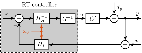
For many practical applications, first order complementary filters are not sufficient. Specifically, a slope of $+2$ at low frequencies for the sensitivity transfer function (enabling accurate tracking of ramp inputs) and a slope of $-2$ for the complementary sensitivity transfer function are often desired. For these cases, the complementary filters analytical formula in Equation eqref:eq:detail_control_cf_2nd_order is proposed.
\begin{subequations}\label{eq:detail_control_cf_2nd_order}
\begin{align} H_L(s) &= \frac{(1+\alpha) (\frac{s}{\omega_0})+1}{\left((\frac{s}{\omega_0})+1\right) \left((\frac{s}{\omega_0})^2 + \alpha (\frac{s}{\omega_0}) + 1\right)}\\ H_H(s) &= \frac{(\frac{s}{\omega_0})^2 \left((\frac{s}{\omega_0})+1+\alpha\right)}{\left((\frac{s}{\omega_0})+1\right) \left((\frac{s}{\omega_0})^2 + \alpha (\frac{s}{\omega_0}) + 1\right)} \end{align}\end{subequations}
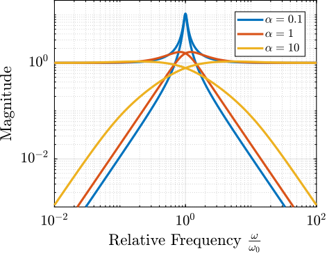
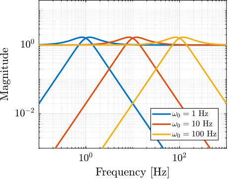
The influence of parameters $\alpha$ and $\omega_0$ on the frequency response of these complementary filters is illustrated in Figure ref:fig:detail_control_cf_analytical_effect. The parameter $\alpha$ primarily affects the damping characteristics near the crossover frequency as well as high and low frequency magnitudes, while $\omega_0$ determines the frequency at which the transition between high-pass and low-pass behavior occurs. These filters can also be implemented in the digital domain with analytical formulas, preserving the ability to adjust $\alpha$ and $\omega_0$ in real-time.
Numerical Example
<<ssec:detail_control_cf_simulations>>
Procedure ignore
To implement the proposed control architecture in practice, the following procedure is proposed:
- Identify the plant to be controlled to obtain the plant model $G$.
- Design the weighting function $w_I$ such that all possible plants $G^\prime$ are contained within the uncertainty set $\Pi_i$.
- Translate performance requirements into upper bounds on the complementary filters as explained in Section ref:ssec:detail_control_cf_trans_perf.
- Design the weighting functions $w_H$ and $w_L$ and generate the complementary filters using $\mathcal{H}_{\infty}\text{-synthesis}$ as described in Section ref:ssec:detail_control_sensor_hinf_method. If the synthesis fails to produce filters satisfying the defined upper bounds, either revise the requirements or develop a more accurate model $G$ that will allow for a smaller $w_I$. For simpler cases, the analytical formulas for complementary filters presented in Section ref:ssec:detail_control_cf_analytical_complementary_filters can be employed.
- If $K(s) = H_H^{-1}(s) G^{-1}(s)$ is not proper, add low-pass filters with sufficiently high corner frequencies to ensure realizability.
Plant ignore
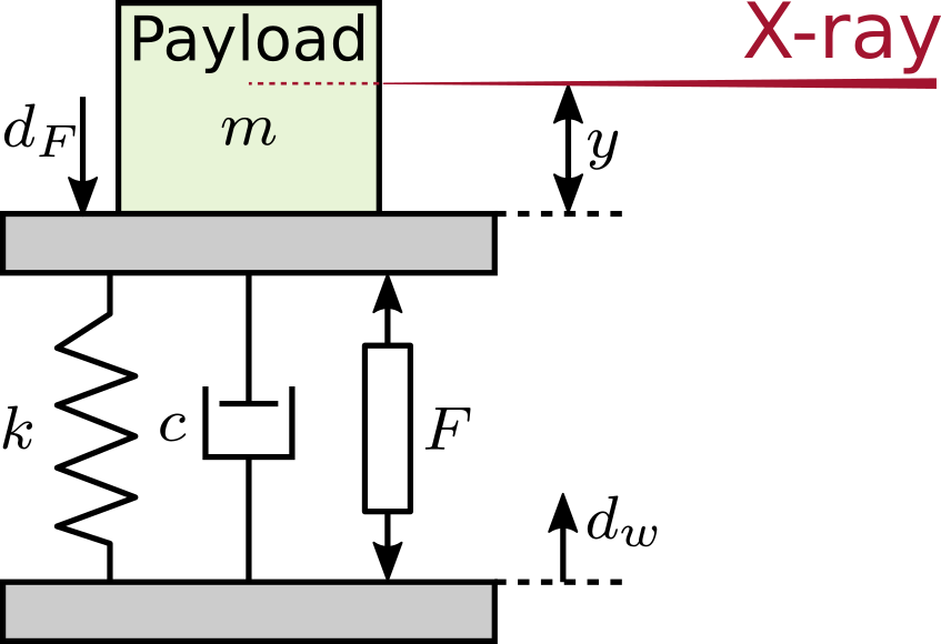
To evaluate this control architecture, a simple test model representative of many synchrotron positioning stages is utilized (Figure ref:fig:detail_control_cf_test_model). In this model, a payload with mass $m$ is positioned on top of a stage. The objective is to accurately position the sample relative to the X-ray beam.
The relative position $y$ between the payload and the X-ray is measured, which typically involves measuring the relative position between the focusing optics and the sample. Various disturbance forces affect positioning stability, including stage vibrations $d_w$ and direct forces applied to the sample $d_F$ (such as cable forces). The positioning stage itself is characterized by stiffness $k$, internal damping $c$, and a controllable force $F$.
The model of the plant $G(s)$ from actuator force $F$ to displacement $y$ is described by Equation eqref:eq:detail_control_cf_test_plant_tf.
\begin{equation}\label{eq:detail_control_cf_test_plant_tf} G(s) = \frac{1}{m s^2 + c s + k}, \quad m = §I{20}{\kg},\ k = 1\si{\N/μ\m},\ c = 10^2\si{\N\per(\m\per\s)}
\end{equation}
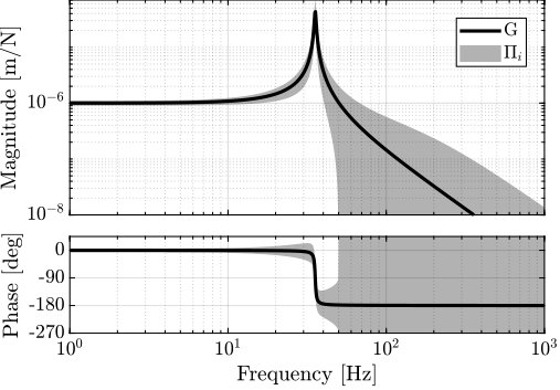
The plant dynamics include uncertainties related to limited support compliance, unmodeled flexible dynamics and payload dynamics. These uncertainties are represented using a multiplicative input uncertainty weight eqref:eq:detail_control_cf_test_plant_uncertainty, which specifies the magnitude of uncertainty as a function of frequency.
\begin{equation}\label{eq:detail_control_cf_test_plant_uncertainty} w_I(s) = 10 ⋅ \frac{(s+100)^2}{(s+1000)^2}
\end{equation}
Figure ref:fig:detail_control_cf_bode_plot_mech_sys illustrates both the nominal plant dynamics and the complete set of possible plants $\Pi_i$ encompassed by the uncertainty model.
Requirements and choice of complementary filters
As discussed in Section ref:ssec:detail_control_cf_trans_perf, nominal performance requirements can be expressed as upper bounds on the shape of the complementary filters. For this example, the requirements are:
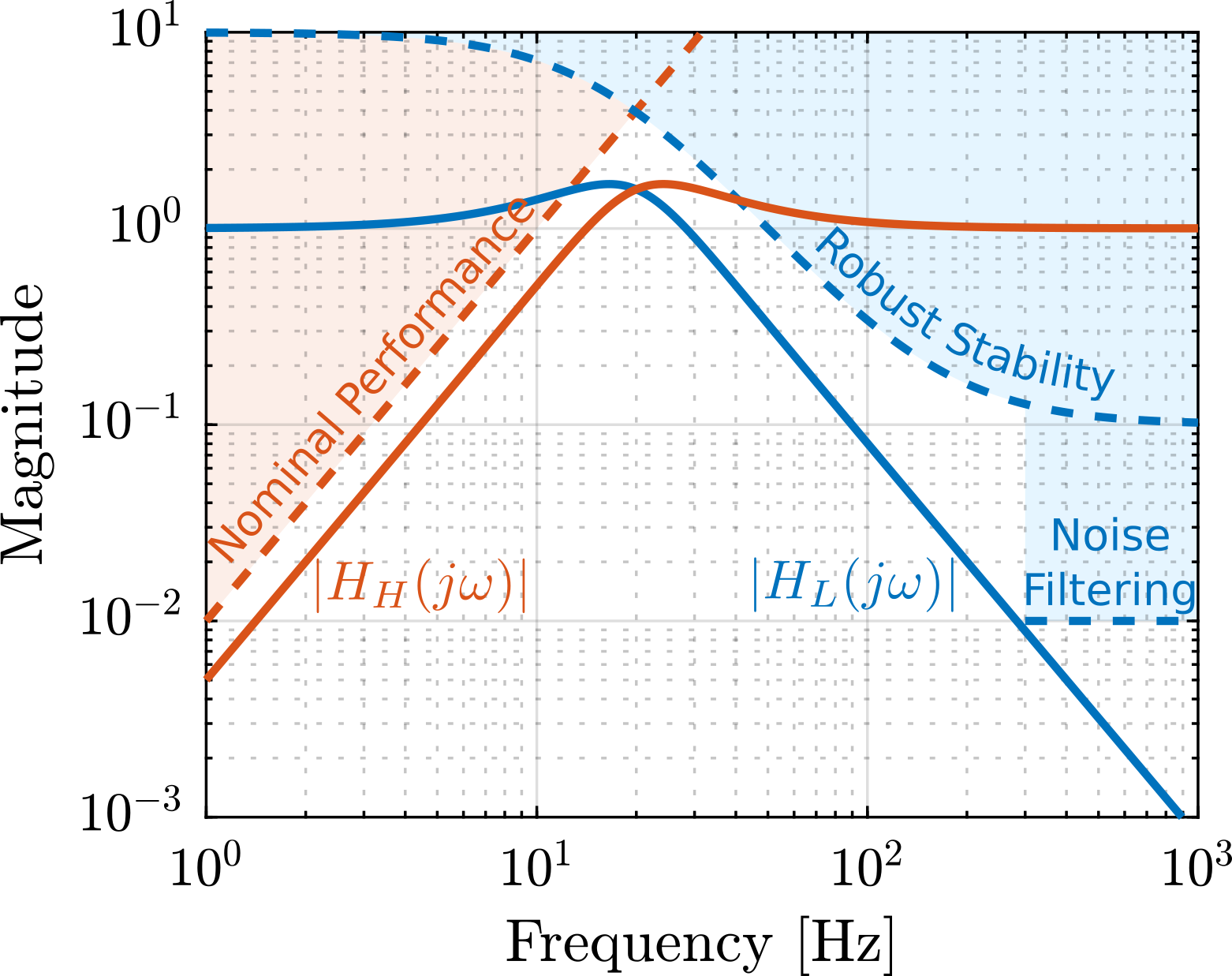
- track ramp inputs (i.e. constant velocity scans) with zero steady-state error: a $+2$ slope at low frequencies for the magnitude of the sensitivity function $|S(j\omega)|$ is required
- filtering of measurement noise above $\SI{300}{Hz}$, where sensor noise is significant (requiring a filtering factor of approximately 100 above this frequency)
- maximizing disturbance rejection
Additionally, robust stability must be ensured, requiring the closed-loop system to remain stable despite the dynamic uncertainties modeled by $w_I$. This condition is satisfied when the magnitude of the low-pass complementary filter $|H_L(j\omega)|$ remains below the inverse of the uncertainty weight magnitude $|w_I(j\omega)|$, as expressed in Equation eqref:eq:detail_control_cf_condition_robust_stability.
Robust performance is achieved when both nominal performance and robust stability conditions are simultaneously satisfied.
All requirements imposed on $H_L$ and $H_H$ are visualized in Figure ref:fig:detail_control_cf_specs_S_T. While $\mathcal{H}_\infty\text{-synthesis}$ could be employed to design the complementary filters, analytical formulas were used for this relatively simple example. The second-order complementary filters from Equation eqref:eq:detail_control_cf_2nd_order were selected with parameters $\alpha = 1$ and $\omega_0 = 2\pi \cdot 20\,\text{Hz}$. There magnitudes are displayed in Figure ref:fig:detail_control_cf_specs_S_T, confirming that these complementary filters are fulfilling the specifications.
Controller analysis
The controller to be implemented takes the form $K(s) = \tilde{G}^{-1}(s) H_H^{-1}(s)$, where $\tilde{G}^{-1}(s)$ represents the plant inverse, which must be both stable and proper. To ensure properness, low-pass filters with high corner frequencies are added as shown in Equation eqref:eq:detail_control_cf_test_plant_inverse.
\begin{equation}\label{eq:detail_control_cf_test_plant_inverse} ~{G}-1(s) = \frac{m s^2 + c s + k}{1 + \frac{s}{2π ⋅ 1000} + ≤ft( \frac{s}{2π ⋅ 1000} \right)^2}
\end{equation}
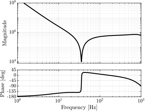
The Bode plot of the controller multiplied by the complementary low-pass filter, $K(s) \cdot H_L(s)$, is presented in Figure ref:fig:detail_control_cf_bode_Kfb. The frequency response reveals several important characteristics:
- The presence of two integrators at low frequencies, enabling accurate tracking of ramp inputs
- A notch at the plant resonance frequency (arising from the plant inverse)
- A lead component near the control bandwidth of approximately 20 Hz, enhancing stability margins
Robustness and Performance analysis
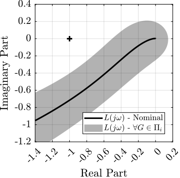
Robust stability is assessed using the Nyquist plot shown in Figure ref:fig:detail_control_cf_nyquist_robustness. Even when considering all possible plants within the uncertainty set, the Nyquist plot remains sufficiently distant from the critical point $(-1,0)$, indicating robust stability with adequate margins.
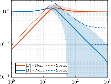
Performance is evaluated by examining the closed-loop sensitivity and complementary sensitivity transfer functions, as illustrated in Figure ref:fig:detail_control_cf_robust_perf. It is shown that the sensitivity transfer function achieves the desired $+2$ slope at low frequencies and that the complementary sensitivity transfer function nominally provides the wanted noise filtering.
Conclusion
In this section, a control architecture in which complementary filters are used for closed-loop shaping has been presented. This approach differs from traditional open-loop shaping in that no controller is manually designed; rather, appropriate complementary filters are selected to achieve the desired closed-loop behavior. The method shares conceptual similarities with mixed-sensitivity $\mathcal{H}_{\infty}\text{-synthesis}$, as both approaches aim to shape closed-loop transfer functions, but with notable distinctions in implementation and complexity.
While $\mathcal{H}_{\infty}\text{-synthesis}$ offers greater flexibility and can be readily generalized to MIMO plants, the presented approach provides a simpler alternative that requires minimal design effort. Implementation only necessitates extracting a model of the plant and selecting appropriate analytical complementary filters, making it particularly interesting for applications where simplicity and intuitive parameter tuning are valued.
Due to time constraints, an extensive literature review comparing this approach with similar existing architectures, such as Internal Model Control cite:&saxena12_advan_inter_model_contr_techn, was not conducted. Consequently, it remains unclear whether the proposed architecture offers significant advantages over existing methods in the literature.
The control architecture has been presented for SISO systems, but can be applied to MIMO systems when sufficient decoupling is achieved. It will be experimentally validated with the NASS during the experimental phase.
Bibliography ignore
\bibliography{dehaeze26_control}
Footnotes
1$n$ corresponds to the number of degrees of freedom, here $n = 3$
