dehaeze21_desig_compl_filte/matlab/index.org

Complementary Filters Shaping Using $\mathcal{H}_\infty$ Synthesis - Matlab Computation

• Introduction
• H-Infinity synthesis of complementary filters
  • Introduction
  • Synthesis Architecture
  • Design of Weighting Function
  • H-Infinity Synthesis
  • Obtained Complementary Filters
• Generating 3 complementary filters
  • Introduction
  • Theory
  • Weights
  • H-Infinity Synthesis
  • Obtained Complementary Filters
• Implement complementary filters for LIGO
  • Introduction
  • Specifications
  • FIR Filter
  • Weights
  • H-Infinity Synthesis
  • Compare FIR and H-Infinity Filters
• Alternative Synthesis
  • Two generalized plants
  • Shaping the Low pass filter or the high pass filter?
• Impose a positive slope at DC or a negative slope at infinite frequency
  • Manually shift zeros to the origin after synthesis
  • Imposing a positive slope at DC during the synthesis phase
  • Imposing a negative slope at infinity frequency during the synthesis phase
• Bibliography

Introduction   ignore

In this document, the design of complementary filters is studied.

One use of complementary filter is described below:

The basic idea of a complementary filter involves taking two or more sensors, filtering out unreliable frequencies for each sensor, and combining the filtered outputs to get a better estimate throughout the entire bandwidth of the system. To achieve this, the sensors included in the filter should complement one another by performing better over specific parts of the system bandwidth.

This document is divided into several sections:

• in section sec:h_inf_synthesis_complementary_filters, the $\mathcal{H}_\infty$ synthesis is used for generating two complementary filters
• in section sec:three_comp_filters, a method using the $\mathcal{H}_\infty$ synthesis is proposed to shape three of more complementary filters
• in section sec:comp_filters_ligo, the $\mathcal{H}_\infty$ synthesis is used and compared with FIR complementary filters used for LIGO

Add the Matlab code use to obtain the results presented in the paper are accessible here and presented below.

H-Infinity synthesis of complementary filters

<<sec:h_inf_synthesis_complementary_filters>>

Introduction   ignore

The Matlab file corresponding to this section is accessible here.

Synthesis Architecture

We here synthesize two complementary filters using the $\mathcal{H}_\infty$ synthesis. The goal is to specify upper bounds on the norms of the two complementary filters $H_1(s)$ and $H_2(s)$ while ensuring their complementary property ($H_1(s) + H_2(s) = 1$).

In order to do so, we use the generalized plant shown on figure fig:h_infinity_robst_fusion where $W_1(s)$ and $W_2(s)$ are weighting transfer functions that will be used to shape $H_1(s)$ and $H_2(s)$ respectively.

$\mathcal{H}_\infty$ synthesis of the complementary filters

The $\mathcal{H}_\infty$ synthesis applied on this generalized plant will give a transfer function $H_2$ (figure fig:h_infinity_robst_fusion) such that the $\mathcal{H}_\infty$ norm of the transfer function from $w$ to $[z_1,\ z_2]$ is less than one: \[ \left\| \begin{array}{c} (1 - H_2(s)) W_1(s) \\ H_2(s) W_2(s) \end{array} \right\|_\infty < 1 \]

Thus, if the above condition is verified, we can define $H_1(s) = 1 - H_2(s)$ and we have that: \[ \left\| \begin{array}{c} H_1(s) W_1(s) \\ H_2(s) W_2(s) \end{array} \right\|_\infty < 1 \] Which is almost (with an maximum error of $\sqrt{2}$) equivalent to:

\begin{align*} |H_1(j\omega)| &< \frac{1}{|W_1(j\omega)|}, \quad \forall \omega \\ |H_2(j\omega)| &< \frac{1}{|W_2(j\omega)|}, \quad \forall \omega \end{align*}

We then see that $W_1(s)$ and $W_2(s)$ can be used to shape both $H_1(s)$ and $H_2(s)$ while ensuring their complementary property by the definition of $H_1(s) = 1 - H_2(s)$.

Design of Weighting Function

A formula is proposed to help the design of the weighting functions:

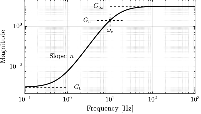
\begin{equation} W(s) = \left( \frac{ \frac{1}{\omega_0} \sqrt{\frac{1 - \left(\frac{G_0}{G_c}\right)^{\frac{2}{n}}}{1 - \left(\frac{G_c}{G_\infty}\right)^{\frac{2}{n}}}} s + \left(\frac{G_0}{G_c}\right)^{\frac{1}{n}} }{ \left(\frac{1}{G_\infty}\right)^{\frac{1}{n}} \frac{1}{\omega_0} \sqrt{\frac{1 - \left(\frac{G_0}{G_c}\right)^{\frac{2}{n}}}{1 - \left(\frac{G_c}{G_\infty}\right)^{\frac{2}{n}}}} s + \left(\frac{1}{G_c}\right)^{\frac{1}{n}} }\right)^n \end{equation}

The parameters permits to specify:

• the low frequency gain: $G_0 = lim_{\omega \to 0} |W(j\omega)|$
• the high frequency gain: $G_\infty = lim_{\omega \to \infty} |W(j\omega)|$
• the absolute gain at $\omega_0$: $G_c = |W(j\omega_0)|$
• the absolute slope between high and low frequency: $n$

The general shape of a weighting function generated using the formula is shown in figure fig:weight_formula.

Gain of the Weighting Function formula

  n = 2; w0 = 2*pi*11; G0 = 1/10; G1 = 1000; Gc = 1/2;
  W1 = (((1/w0)*sqrt((1-(G0/Gc)^(2/n))/(1-(Gc/G1)^(2/n)))*s + (G0/Gc)^(1/n))/((1/G1)^(1/n)*(1/w0)*sqrt((1-(G0/Gc)^(2/n))/(1-(Gc/G1)^(2/n)))*s + (1/Gc)^(1/n)))^n;

  n = 3; w0 = 2*pi*10; G0 = 1000; G1 = 0.1; Gc = 1/2;
  W2 = (((1/w0)*sqrt((1-(G0/Gc)^(2/n))/(1-(Gc/G1)^(2/n)))*s + (G0/Gc)^(1/n))/((1/G1)^(1/n)*(1/w0)*sqrt((1-(G0/Gc)^(2/n))/(1-(Gc/G1)^(2/n)))*s + (1/Gc)^(1/n)))^n;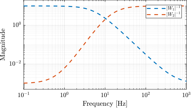

Weights on the complementary filters $W_1$ and $W_2$ and the associated performance weights

H-Infinity Synthesis

We define the generalized plant $P$ on matlab.

  P = [W1 -W1;
       0   W2;
       1   0];

And we do the $\mathcal{H}_\infty$ synthesis using the hinfsyn command.

  [H2, ~, gamma, ~] = hinfsyn(P, 1, 1,'TOLGAM', 0.001, 'METHOD', 'ric', 'DISPLAY', 'on');

[H2, ~, gamma, ~] = hinfsyn(P, 1, 1,'TOLGAM', 0.001, 'METHOD', 'ric', 'DISPLAY', 'on');
Resetting value of Gamma min based on D_11, D_12, D_21 terms

Test bounds:      0.1000 <  gamma  <=   1050.0000

  gamma    hamx_eig  xinf_eig  hamy_eig   yinf_eig   nrho_xy   p/f
1.050e+03   2.8e+01   2.4e-07   4.1e+00    0.0e+00    0.0000    p
  525.050   2.8e+01   2.4e-07   4.1e+00    0.0e+00    0.0000    p
  262.575   2.8e+01   2.4e-07   4.1e+00    0.0e+00    0.0000    p
  131.337   2.8e+01   2.4e-07   4.1e+00   -1.0e-13    0.0000    p
   65.719   2.8e+01   2.4e-07   4.1e+00   -9.5e-14    0.0000    p
   32.909   2.8e+01   2.4e-07   4.1e+00    0.0e+00    0.0000    p
   16.505   2.8e+01   2.4e-07   4.1e+00   -1.0e-13    0.0000    p
    8.302   2.8e+01   2.4e-07   4.1e+00   -7.2e-14    0.0000    p
    4.201   2.8e+01   2.4e-07   4.1e+00   -2.5e-25    0.0000    p
    2.151   2.7e+01   2.4e-07   4.1e+00   -3.8e-14    0.0000    p
    1.125   2.6e+01   2.4e-07   4.1e+00   -5.4e-24    0.0000    p
    0.613   2.3e+01 -3.7e+01#  4.1e+00    0.0e+00    0.0000    f
    0.869   2.6e+01 -3.7e+02#  4.1e+00    0.0e+00    0.0000    f
    0.997   2.6e+01 -1.1e+04#  4.1e+00    0.0e+00    0.0000    f
    1.061   2.6e+01   2.4e-07   4.1e+00    0.0e+00    0.0000    p
    1.029   2.6e+01   2.4e-07   4.1e+00    0.0e+00    0.0000    p
    1.013   2.6e+01   2.4e-07   4.1e+00    0.0e+00    0.0000    p
    1.005   2.6e+01   2.4e-07   4.1e+00    0.0e+00    0.0000    p
    1.001   2.6e+01 -3.1e+04#  4.1e+00   -3.8e-14    0.0000    f
    1.003   2.6e+01 -2.8e+05#  4.1e+00    0.0e+00    0.0000    f
    1.004   2.6e+01   2.4e-07   4.1e+00   -5.8e-24    0.0000    p
    1.004   2.6e+01   2.4e-07   4.1e+00    0.0e+00    0.0000    p

 Gamma value achieved:     1.0036

We then define the high pass filter $H_1 = 1 - H_2$. The bode plot of both $H_1$ and $H_2$ is shown on figure fig:hinf_filters_results.

  H1 = 1 - H2;

Obtained Complementary Filters

The obtained complementary filters are shown on figure fig:hinf_filters_results.

Obtained complementary filters using $\mathcal{H}_\infty$ synthesis

Generating 3 complementary filters

<<sec:three_comp_filters>>

Introduction   ignore

The Matlab file corresponding to this section is accessible here.

Theory

We want:

\begin{align*} & |H_1(j\omega)| < 1/|W_1(j\omega)|, \quad \forall\omega\\ & |H_2(j\omega)| < 1/|W_2(j\omega)|, \quad \forall\omega\\ & |H_3(j\omega)| < 1/|W_3(j\omega)|, \quad \forall\omega\\ & H_1(s) + H_2(s) + H_3(s) = 1 \end{align*}

For that, we use the $\mathcal{H}_\infty$ synthesis with the architecture shown on figure fig:comp_filter_three_hinf.

Generalized architecture for generating 3 complementary filters

The $\mathcal{H}_\infty$ objective is:

\begin{align*} & |(1 - H_2(j\omega) - H_3(j\omega)) W_1(j\omega)| < 1, \quad \forall\omega\\ & |H_2(j\omega) W_2(j\omega)| < 1, \quad \forall\omega\\ & |H_3(j\omega) W_3(j\omega)| < 1, \quad \forall\omega\\ \end{align*}

And thus if we choose $H_1 = 1 - H_2 - H_3$ we have solved the problem.

Weights

First we define the weights.

  n = 2; w0 = 2*pi*1; G0 = 1/10; G1 = 1000; Gc = 1/2;
  W1 = (((1/w0)*sqrt((1-(G0/Gc)^(2/n))/(1-(Gc/G1)^(2/n)))*s + (G0/Gc)^(1/n))/((1/G1)^(1/n)*(1/w0)*sqrt((1-(G0/Gc)^(2/n))/(1-(Gc/G1)^(2/n)))*s + (1/Gc)^(1/n)))^n;

  W2 = 0.22*(1 + s/2/pi/1)^2/(sqrt(1e-4) + s/2/pi/1)^2*(1 + s/2/pi/10)^2/(1 + s/2/pi/1000)^2;

  n = 3; w0 = 2*pi*10; G0 = 1000; G1 = 0.1; Gc = 1/2;
  W3 = (((1/w0)*sqrt((1-(G0/Gc)^(2/n))/(1-(Gc/G1)^(2/n)))*s + (G0/Gc)^(1/n))/((1/G1)^(1/n)*(1/w0)*sqrt((1-(G0/Gc)^(2/n))/(1-(Gc/G1)^(2/n)))*s + (1/Gc)^(1/n)))^n;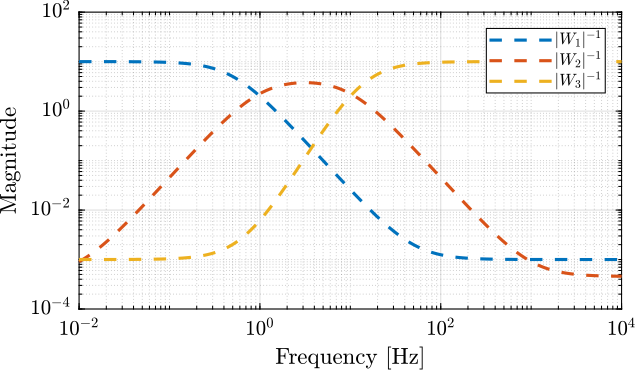

Three weighting functions used for the $\mathcal{H}_\infty$ synthesis of the complementary filters

H-Infinity Synthesis

Then we create the generalized plant P.

  P = [W1 -W1 -W1;
       0   W2  0 ;
       0   0   W3;
       1   0   0];

And we do the $\mathcal{H}_\infty$ synthesis.

  [H, ~, gamma, ~] = hinfsyn(P, 1, 2,'TOLGAM', 0.001, 'METHOD', 'ric', 'DISPLAY', 'on');

[H, ~, gamma, ~] = hinfsyn(P, 1, 2,'TOLGAM', 0.001, 'METHOD', 'ric', 'DISPLAY', 'on');
Resetting value of Gamma min based on D_11, D_12, D_21 terms

Test bounds:      0.1000 <  gamma  <=   1050.0000

  gamma    hamx_eig  xinf_eig  hamy_eig   yinf_eig   nrho_xy   p/f
1.050e+03   3.2e+00   4.5e-13   6.3e-02   -1.2e-11    0.0000    p
  525.050   3.2e+00   1.3e-13   6.3e-02    0.0e+00    0.0000    p
  262.575   3.2e+00   2.1e-12   6.3e-02   -1.5e-13    0.0000    p
  131.337   3.2e+00   1.1e-12   6.3e-02   -7.2e-29    0.0000    p
   65.719   3.2e+00   2.0e-12   6.3e-02    0.0e+00    0.0000    p
   32.909   3.2e+00   7.4e-13   6.3e-02   -5.9e-13    0.0000    p
   16.505   3.2e+00   1.4e-12   6.3e-02    0.0e+00    0.0000    p
    8.302   3.2e+00   1.6e-12   6.3e-02    0.0e+00    0.0000    p
    4.201   3.2e+00   1.6e-12   6.3e-02    0.0e+00    0.0000    p
    2.151   3.2e+00   1.6e-12   6.3e-02    0.0e+00    0.0000    p
    1.125   3.2e+00   2.8e-12   6.3e-02    0.0e+00    0.0000    p
    0.613   3.0e+00 -2.5e+03#  6.3e-02    0.0e+00    0.0000    f
    0.869   3.1e+00 -2.9e+01#  6.3e-02    0.0e+00    0.0000    f
    0.997   3.2e+00   1.9e-12   6.3e-02    0.0e+00    0.0000    p
    0.933   3.1e+00 -6.9e+02#  6.3e-02    0.0e+00    0.0000    f
    0.965   3.1e+00 -3.0e+03#  6.3e-02    0.0e+00    0.0000    f
    0.981   3.1e+00 -8.6e+03#  6.3e-02    0.0e+00    0.0000    f
    0.989   3.2e+00 -2.7e+04#  6.3e-02    0.0e+00    0.0000    f
    0.993   3.2e+00 -5.7e+05#  6.3e-02    0.0e+00    0.0000    f
    0.995   3.2e+00   2.2e-12   6.3e-02    0.0e+00    0.0000    p
    0.994   3.2e+00   1.6e-12   6.3e-02    0.0e+00    0.0000    p
    0.994   3.2e+00   1.0e-12   6.3e-02    0.0e+00    0.0000    p

 Gamma value achieved:     0.9936

Obtained Complementary Filters

The obtained filters are:

  H2 = tf(H(1));
  H3 = tf(H(2));
  H1 = 1 - H2 - H3;

The three complementary filters obtained after $\mathcal{H}_\infty$ synthesis

Implement complementary filters for LIGO

<<sec:comp_filters_ligo>>

Introduction   ignore

The Matlab file corresponding to this section is accessible here.

Let's try to design complementary filters that are corresponding to the complementary filters design for the LIGO and described in cite:hua05_low_ligo.

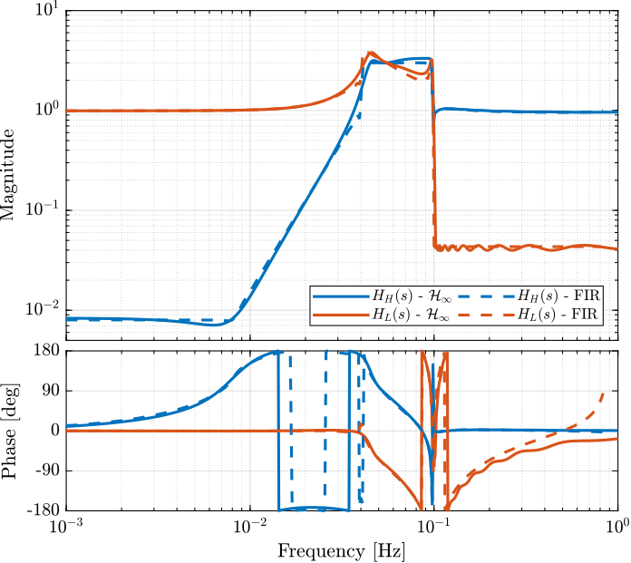
The FIR complementary filters designed in cite:hua05_low_ligo are of order 512.

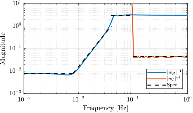
Specifications

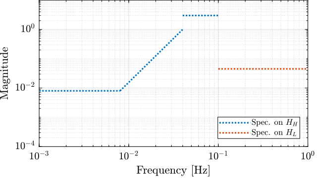
The specifications for the filters are:

1. From $0$ to $0.008\text{ Hz}$,the magnitude of the filter’s transfer function should be less than or equal to $8 \times 10^{-3}$
2. From $0.008\text{ Hz}$ to $0.04\text{ Hz}$, it attenuates the input signal proportional to frequency cubed
3. Between $0.04\text{ Hz}$ and $0.1\text{ Hz}$, the magnitude of the transfer function should be less than 3
4. Above $0.1\text{ Hz}$, the maximum of the magnitude of the complement filter should be as close to zero as possible. In our system, we would like to have the magnitude of the complementary filter to be less than $0.1$. As the filters obtained in cite:hua05_low_ligo have a magnitude of $0.045$, we will set that as our requirement

The specifications are translated in upper bounds of the complementary filters are shown on figure fig:ligo_specifications.

Specification for the LIGO complementary filters

TODO FIR Filter

We here try to implement the FIR complementary filter synthesis as explained in cite:hua05_low_ligo. For that, we use the CVX matlab Toolbox.

We setup the CVX toolbox and use the SeDuMi solver.

  cvx_startup;
  cvx_solver sedumi;

We define the frequency vectors on which we will constrain the norm of the FIR filter.

  w1 = 0:4.06e-4:0.008;
  w2 = 0.008:4.06e-4:0.04;
  w3 = 0.04:8.12e-4:0.1;
  w4 = 0.1:8.12e-4:0.83;

We then define the order of the FIR filter.

  n = 512;

  A1 = [ones(length(w1),1),  cos(kron(w1'.*(2*pi),[1:n-1]))];
  A2 = [ones(length(w2),1),  cos(kron(w2'.*(2*pi),[1:n-1]))];
  A3 = [ones(length(w3),1),  cos(kron(w3'.*(2*pi),[1:n-1]))];
  A4 = [ones(length(w4),1),  cos(kron(w4'.*(2*pi),[1:n-1]))];

  B1 = [zeros(length(w1),1), sin(kron(w1'.*(2*pi),[1:n-1]))];
  B2 = [zeros(length(w2),1), sin(kron(w2'.*(2*pi),[1:n-1]))];
  B3 = [zeros(length(w3),1), sin(kron(w3'.*(2*pi),[1:n-1]))];
  B4 = [zeros(length(w4),1), sin(kron(w4'.*(2*pi),[1:n-1]))];

We run the convex optimization.

  cvx_begin

  variable y(n+1,1)

  % t
  maximize(-y(1))

  for i = 1:length(w1)
      norm([0 A1(i,:); 0 B1(i,:)]*y) <= 8e-3;
  end

  for  i = 1:length(w2)
      norm([0 A2(i,:); 0 B2(i,:)]*y) <= 8e-3*(2*pi*w2(i)/(0.008*2*pi))^3;
  end

  for i = 1:length(w3)
      norm([0 A3(i,:); 0 B3(i,:)]*y) <= 3;
  end

  for i = 1:length(w4)
      norm([[1 0]'- [0 A4(i,:); 0 B4(i,:)]*y]) <= y(1);
  end

  cvx_end

  h = y(2:end);

cvx_begin
variable y(n+1,1)
% t
maximize(-y(1))
for i = 1:length(w1)
    norm([0 A1(i,:); 0 B1(i,:)]*y) <= 8e-3;
end
for  i = 1:length(w2)
    norm([0 A2(i,:); 0 B2(i,:)]*y) <= 8e-3*(2*pi*w2(i)/(0.008*2*pi))^3;
end
for i = 1:length(w3)
    norm([0 A3(i,:); 0 B3(i,:)]*y) <= 3;
end
for i = 1:length(w4)
    norm([[1 0]'- [0 A4(i,:); 0 B4(i,:)]*y]) <= y(1);
end
cvx_end

Calling SeDuMi 1.34: 4291 variables, 1586 equality constraints
   For improved efficiency, SeDuMi is solving the dual problem.
------------------------------------------------------------
SeDuMi 1.34 (beta) by AdvOL, 2005-2008 and Jos F. Sturm, 1998-2003.
Alg = 2: xz-corrector, Adaptive Step-Differentiation, theta = 0.250, beta = 0.500
eqs m = 1586, order n = 3220, dim = 4292, blocks = 1073
nnz(A) = 1100727 + 0, nnz(ADA) = 1364794, nnz(L) = 683190
 it :     b*y       gap    delta  rate   t/tP*  t/tD*   feas cg cg  prec
  0 :            4.11E+02 0.000
  1 :  -2.58E+00 1.25E+02 0.000 0.3049 0.9000 0.9000   4.87  1  1  3.0E+02
  2 :  -2.36E+00 3.90E+01 0.000 0.3118 0.9000 0.9000   1.83  1  1  6.6E+01
  3 :  -1.69E+00 1.31E+01 0.000 0.3354 0.9000 0.9000   1.76  1  1  1.5E+01
  4 :  -8.60E-01 7.10E+00 0.000 0.5424 0.9000 0.9000   2.48  1  1  4.8E+00
  5 :  -4.91E-01 5.44E+00 0.000 0.7661 0.9000 0.9000   3.12  1  1  2.5E+00
  6 :  -2.96E-01 3.88E+00 0.000 0.7140 0.9000 0.9000   2.62  1  1  1.4E+00
  7 :  -1.98E-01 2.82E+00 0.000 0.7271 0.9000 0.9000   2.14  1  1  8.5E-01
  8 :  -1.39E-01 2.00E+00 0.000 0.7092 0.9000 0.9000   1.78  1  1  5.4E-01
  9 :  -9.99E-02 1.30E+00 0.000 0.6494 0.9000 0.9000   1.51  1  1  3.3E-01
 10 :  -7.57E-02 8.03E-01 0.000 0.6175 0.9000 0.9000   1.31  1  1  2.0E-01
 11 :  -5.99E-02 4.22E-01 0.000 0.5257 0.9000 0.9000   1.17  1  1  1.0E-01
 12 :  -5.28E-02 2.45E-01 0.000 0.5808 0.9000 0.9000   1.08  1  1  5.9E-02
 13 :  -4.82E-02 1.28E-01 0.000 0.5218 0.9000 0.9000   1.05  1  1  3.1E-02
 14 :  -4.56E-02 5.65E-02 0.000 0.4417 0.9045 0.9000   1.02  1  1  1.4E-02
 15 :  -4.43E-02 2.41E-02 0.000 0.4265 0.9004 0.9000   1.01  1  1  6.0E-03
 16 :  -4.37E-02 8.90E-03 0.000 0.3690 0.9070 0.9000   1.00  1  1  2.3E-03
 17 :  -4.35E-02 3.24E-03 0.000 0.3641 0.9164 0.9000   1.00  1  1  9.5E-04
 18 :  -4.34E-02 1.55E-03 0.000 0.4788 0.9086 0.9000   1.00  1  1  4.7E-04
 19 :  -4.34E-02 8.77E-04 0.000 0.5653 0.9169 0.9000   1.00  1  1  2.8E-04
 20 :  -4.34E-02 5.05E-04 0.000 0.5754 0.9034 0.9000   1.00  1  1  1.6E-04
 21 :  -4.34E-02 2.94E-04 0.000 0.5829 0.9136 0.9000   1.00  1  1  9.9E-05
 22 :  -4.34E-02 1.63E-04 0.015 0.5548 0.9000 0.0000   1.00  1  1  6.6E-05
 23 :  -4.33E-02 9.42E-05 0.000 0.5774 0.9053 0.9000   1.00  1  1  3.9E-05
 24 :  -4.33E-02 6.27E-05 0.000 0.6658 0.9148 0.9000   1.00  1  1  2.6E-05
 25 :  -4.33E-02 3.75E-05 0.000 0.5972 0.9187 0.9000   1.00  1  1  1.6E-05
 26 :  -4.33E-02 1.89E-05 0.000 0.5041 0.9117 0.9000   1.00  1  1  8.6E-06
 27 :  -4.33E-02 9.72E-06 0.000 0.5149 0.9050 0.9000   1.00  1  1  4.5E-06
 28 :  -4.33E-02 2.94E-06 0.000 0.3021 0.9194 0.9000   1.00  1  1  1.5E-06
 29 :  -4.33E-02 9.73E-07 0.000 0.3312 0.9189 0.9000   1.00  2  2  5.3E-07
 30 :  -4.33E-02 2.82E-07 0.000 0.2895 0.9063 0.9000   1.00  2  2  1.6E-07
 31 :  -4.33E-02 8.05E-08 0.000 0.2859 0.9049 0.9000   1.00  2  2  4.7E-08
 32 :  -4.33E-02 1.43E-08 0.000 0.1772 0.9059 0.9000   1.00  2  2  8.8E-09

iter seconds digits       c*x               b*y
 32     49.4   6.8 -4.3334083581e-02 -4.3334090214e-02
|Ax-b| =   3.7e-09, [Ay-c]_+ =   1.1E-10, |x|=  1.0e+00, |y|=  2.6e+00

Detailed timing (sec)
   Pre          IPM          Post
3.902E+00    4.576E+01    1.035E-02
Max-norms: ||b||=1, ||c|| = 3,
Cholesky |add|=0, |skip| = 0, ||L.L|| = 4.26267.
------------------------------------------------------------
Status: Solved
Optimal value (cvx_optval): -0.0433341
h = y(2:end);

Finally, we compute the filter response over the frequency vector defined and the result is shown on figure fig:fir_filter_ligo which is very close to the filters obtain in cite:hua05_low_ligo.

  w = [w1 w2 w3 w4];
  H = [exp(-j*kron(w'.*2*pi,[0:n-1]))]*h;

FIR Complementary filters obtain after convex optimization

Weights

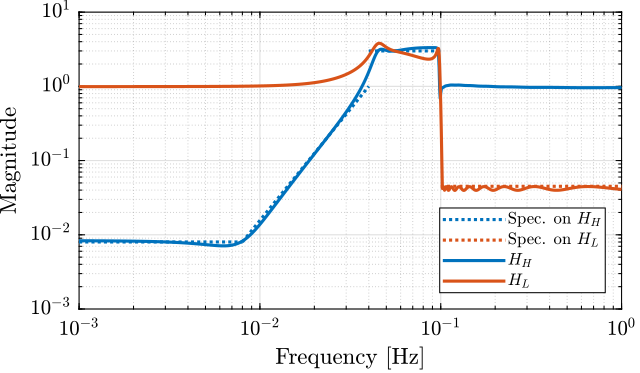
We design weights that will be used for the $\mathcal{H}_\infty$ synthesis of the complementary filters. These weights will determine the order of the obtained filters. Here are the requirements on the filters:

• reasonable order
• to be as close as possible to the specified upper bounds
• stable minimum phase

The bode plot of the weights is shown on figure fig:ligo_weights.

Weights for the $\mathcal{H}_\infty$ synthesis

H-Infinity Synthesis

We define the generalized plant as shown on figure fig:h_infinity_robst_fusion.

  P = [0   wL;
       wH -wH;
       1   0];

And we do the $\mathcal{H}_\infty$ synthesis using the hinfsyn command.

  [Hl, ~, gamma, ~] = hinfsyn(P, 1, 1,'TOLGAM', 0.001, 'METHOD', 'ric', 'DISPLAY', 'on');

[Hl, ~, gamma, ~] = hinfsyn(P, 1, 1,'TOLGAM', 0.001, 'METHOD', 'ric', 'DISPLAY', 'on');
Resetting value of Gamma min based on D_11, D_12, D_21 terms

Test bounds:      0.3276 <  gamma  <=      1.8063

  gamma    hamx_eig  xinf_eig  hamy_eig   yinf_eig   nrho_xy   p/f
    1.806   1.4e-02 -1.7e-16   3.6e-03   -4.8e-12    0.0000    p
    1.067   1.3e-02 -4.2e-14   3.6e-03   -1.9e-12    0.0000    p
    0.697   1.3e-02 -3.0e-01#  3.6e-03   -3.5e-11    0.0000    f
    0.882   1.3e-02 -9.5e-01#  3.6e-03   -1.2e-34    0.0000    f
    0.975   1.3e-02 -2.7e+00#  3.6e-03   -1.6e-12    0.0000    f
    1.021   1.3e-02 -8.7e+00#  3.6e-03   -4.5e-16    0.0000    f
    1.044   1.3e-02 -6.5e-14   3.6e-03   -3.0e-15    0.0000    p
    1.032   1.3e-02 -1.8e+01#  3.6e-03    0.0e+00    0.0000    f
    1.038   1.3e-02 -3.8e+01#  3.6e-03    0.0e+00    0.0000    f
    1.041   1.3e-02 -8.3e+01#  3.6e-03   -2.9e-33    0.0000    f
    1.042   1.3e-02 -1.9e+02#  3.6e-03   -3.4e-11    0.0000    f
    1.043   1.3e-02 -5.3e+02#  3.6e-03   -7.5e-13    0.0000    f

 Gamma value achieved:     1.0439

The high pass filter is defined as $H_H = 1 - H_L$.

  Hh = 1 - Hl;

The size of the filters is shown below.

size(Hh), size(Hl)
State-space model with 1 outputs, 1 inputs, and 27 states.
State-space model with 1 outputs, 1 inputs, and 27 states.

The bode plot of the obtained filters as shown on figure fig:hinf_synthesis_ligo_results.

Obtained complementary filters using the $\mathcal{H}_\infty$ synthesis

TODO Compare FIR and H-Infinity Filters

Let's now compare the FIR filters designed in cite:hua05_low_ligo and the one obtained with the $\mathcal{H}_\infty$ synthesis on figure fig:comp_fir_ligo_hinf.

Comparison between the FIR filters developped for LIGO and the $\mathcal{H}_\infty$ complementary filters

Alternative Synthesis

Two generalized plants

In order to synthesize the complementary filter using the proposed method, we can use two alternative generalized plant as shown in Figures fig:h_infinity_arch_1 and fig:h_infinity_arch_2.

\begin{equation} P_1 = \begin{bmatrix} W_1 & -W_1 \\ 0 & W_2 \\ 1 & 0 \end{bmatrix} \end{equation}

  \begin{tikzpicture}
     \node[block={4.5cm}{3.0cm}, fill=black!20!white, dashed] (P) {};
     \node[above] at (P.north) {$P_1(s)$};

     \coordinate[] (inputw)  at ($(P.south west)!0.75!(P.north west) + (-0.7, 0)$);
     \coordinate[] (inputu)  at ($(P.south west)!0.35!(P.north west) + (-0.7, 0)$);

     \coordinate[] (output1) at ($(P.south east)!0.75!(P.north east) + ( 0.7, 0)$);
     \coordinate[] (output2) at ($(P.south east)!0.35!(P.north east) + ( 0.7, 0)$);
     \coordinate[] (outputv) at ($(P.south east)!0.1!(P.north east) + ( 0.7, 0)$);

     \node[block, left=1.4 of output1] (W1){$W_1(s)$};
     \node[block, left=1.4 of output2] (W2){$W_2(s)$};
     \node[addb={+}{}{}{}{-}, left=of W1] (sub) {};

     \node[block, below=0.3 of P] (H2) {$H_2(s)$};

     \draw[->] (inputw) node[above right]{$w$} -- (sub.west);
     \draw[->] (H2.west) -| ($(inputu)+(0.35, 0)$) node[above]{$u$} -- (W2.west);
     \draw[->] (inputu-|sub) node[branch]{} -- (sub.south);
     \draw[->] (sub.east) -- (W1.west);
     \draw[->] ($(sub.west)+(-0.6, 0)$) node[branch]{} |- ($(outputv)+(-0.35, 0)$) node[above]{$v$} |- (H2.east);
     \draw[->] (W1.east) -- (output1)node[above left]{$z_1$};
     \draw[->] (W2.east) -- (output2)node[above left]{$z_2$};
  \end{tikzpicture}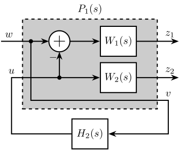

Complementary Filter Synthesis - Conf 1

\begin{equation} P_2 = \begin{bmatrix} 0 & W_1 & 1 \\ W_2 & -W_1 & 0 \end{bmatrix} \end{equation}

  \begin{tikzpicture}
     \node[block={4.5cm}{4.5cm}, fill=black!20!white, dashed] (P) {};
     \node[above] at (P.north) {$P_2(s)$};

     \coordinate[] (input2) at ($(P.south west)!0.85!(P.north west) + (-0.7, 0)$);
     \coordinate[] (input1) at ($(P.south west)!0.55!(P.north west) + (-0.7, 0)$);
     \coordinate[] (inputu) at ($(P.south west)!0.3!( P.north west) + (-0.7, 0)$);

     \coordinate[] (outputz) at ($(P.south east)!0.3!(P.north east) + (0.7, 0)$);
     \coordinate[] (outputv) at ($(P.south east)!0.1!(P.north east) + (0.7, 0)$);

     \node[block, right=1.4 of input2] (W2){$W_2(s)$};
     \node[block, right=1.4 of input1] (W1){$W_1(s)$};
     \node[addb={+}{-}{}{}{}, right=of W1] (sub) {};
     \node[addb, left=2.5 of outputz] (add) {};

     \node[block, below=0.3 of P] (H2) {$H_2(s)$};

     \draw[->] (input2) node[above right]{$w_2$} -- (W2.west);
     \draw[->] (input1) node[above right]{$w_1$} -- (W1.west);
     \draw[->] (W2.east) -| (sub.north);
     \draw[->] (W1.east) -- (sub.west);
     \draw[->] (W1-|add)node[branch]{} -- (add.north);
     \draw[->] (sub.south) |- (outputv) node[above left]{$v$} |- (H2.east);
     \draw[->] (H2.west) -| (inputu) node[above right]{$u$} -- (add.west);
     \draw[->] (add.east) -- (outputz) node[above left]{$z$};
  \end{tikzpicture}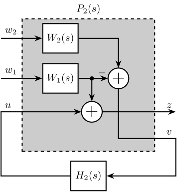

Complementary Filter Synthesis - Conf 2

Let's run the $\mathcal{H}_\infty$ synthesis for both generalized plant using the same weights and see if the obtained filters are the same:

  n = 2; w0 = 2*pi*11; G0 = 1/10; G1 = 1000; Gc = 1/2;
  W1 = (((1/w0)*sqrt((1-(G0/Gc)^(2/n))/(1-(Gc/G1)^(2/n)))*s + (G0/Gc)^(1/n))/((1/G1)^(1/n)*(1/w0)*sqrt((1-(G0/Gc)^(2/n))/(1-(Gc/G1)^(2/n)))*s + (1/Gc)^(1/n)))^n;

  n = 3; w0 = 2*pi*10; G0 = 1000; G1 = 0.1; Gc = 1/2;
  W2 = (((1/w0)*sqrt((1-(G0/Gc)^(2/n))/(1-(Gc/G1)^(2/n)))*s + (G0/Gc)^(1/n))/((1/G1)^(1/n)*(1/w0)*sqrt((1-(G0/Gc)^(2/n))/(1-(Gc/G1)^(2/n)))*s + (1/Gc)^(1/n)))^n;

  P1 = [W1 -W1;
        0   W2;
        1   0];

  [H2, ~, gamma, ~] = hinfsyn(P1, 1, 1,'TOLGAM', 0.001, 'METHOD', 'ric', 'DISPLAY', 'on');

[H2, ~, gamma, ~] = hinfsyn(P1, 1, 1,'TOLGAM', 0.001, 'METHOD', 'ric', 'DISPLAY', 'on');

  Test bounds:  0.3263 <=  gamma  <=  1000

    gamma        X>=0        Y>=0       rho(XY)<1    p/f
  1.807e+01     1.4e-07     0.0e+00     1.185e-18     p
  2.428e+00     1.5e-07     0.0e+00     1.285e-18     p
  8.902e-01    -2.9e+02 #  -7.1e-17     5.168e-19     f
  1.470e+00     1.5e-07     0.0e+00     1.462e-14     p
  1.144e+00     1.5e-07     0.0e+00     1.260e-14     p
  1.009e+00     1.5e-07     0.0e+00     4.120e-13     p
  9.478e-01    -6.8e+02 #  -2.4e-17     1.449e-14     f
  9.780e-01    -1.6e+03 #  -7.3e-17     6.791e-14     f
  9.934e-01    -4.2e+03 #  -1.2e-16     3.524e-14     f
  1.001e+00    -2.0e+04 #  -2.3e-17     5.717e-20     f
  1.005e+00     1.5e-07     0.0e+00     8.953e-18     p
  1.003e+00    -2.2e+05 #  -1.8e-17     3.225e-12     f
  1.004e+00     1.5e-07     0.0e+00     2.445e-12     p
  Limiting gains...
  1.004e+00     1.6e-07     0.0e+00     5.811e-18     p

  Best performance (actual): 1.004

  P2 = [0   W1 1;
        W2 -W1 0];

  [H2b, ~, gamma, ~] = hinfsyn(P2, 1, 1,'TOLGAM', 0.001, 'METHOD', 'ric', 'DISPLAY', 'on');

[H2b, ~, gamma, ~] = hinfsyn(P2, 1, 1,'TOLGAM', 0.001, 'METHOD', 'ric', 'DISPLAY', 'on');

  Test bounds:  0.3263 <=  gamma  <=  1000

    gamma        X>=0        Y>=0       rho(XY)<1    p/f
  1.807e+01     0.0e+00     1.4e-07     2.055e-16     p
  2.428e+00     0.0e+00     1.4e-07     1.894e-18     p
  8.902e-01    -2.1e-16    -2.7e+02 #   1.466e-16     f
  1.470e+00     0.0e+00     1.4e-07     4.118e-16     p
  1.144e+00     0.0e+00     1.5e-07     2.105e-18     p
  1.009e+00     0.0e+00     1.5e-07     2.590e-13     p
  9.478e-01    -9.5e-17    -6.3e+02 #   1.663e-19     f
  9.780e-01    -1.1e-16    -1.5e+03 #   1.546e-14     f
  9.934e-01    -2.8e-17    -4.0e+03 #   3.934e-14     f
  1.001e+00    -3.1e-17    -1.9e+04 #   1.191e-19     f
  1.005e+00     0.0e+00     1.5e-07     1.443e-12     p
  1.003e+00    -8.3e-17    -2.1e+05 #   8.807e-13     f
  1.004e+00     0.0e+00     1.5e-07     1.459e-15     p
  Limiting gains...
  1.004e+00     0.0e+00     1.5e-07     9.086e-19     p

  Best performance (actual): 1.004

And indeed, we can see that the exact same filters are obtained (Figure fig:hinf_comp_P1_P2_syn).

Comparison of $H_2(s)$ when using $P_1(s)$ or $P_2(s)$

Shaping the Low pass filter or the high pass filter?

Let's see if there is a difference by explicitly shaping $H_1(s)$ or $H_2(s)$.

  n = 2; w0 = 2*pi*11; G0 = 1/10; G1 = 1000; Gc = 1/2;
  W1 = (((1/w0)*sqrt((1-(G0/Gc)^(2/n))/(1-(Gc/G1)^(2/n)))*s + (G0/Gc)^(1/n))/((1/G1)^(1/n)*(1/w0)*sqrt((1-(G0/Gc)^(2/n))/(1-(Gc/G1)^(2/n)))*s + (1/Gc)^(1/n)))^n;

  n = 3; w0 = 2*pi*10; G0 = 1000; G1 = 0.1; Gc = 1/2;
  W2 = (((1/w0)*sqrt((1-(G0/Gc)^(2/n))/(1-(Gc/G1)^(2/n)))*s + (G0/Gc)^(1/n))/((1/G1)^(1/n)*(1/w0)*sqrt((1-(G0/Gc)^(2/n))/(1-(Gc/G1)^(2/n)))*s + (1/Gc)^(1/n)))^n;

Let's first synthesize $H_1(s)$:

  P1 = [W2 -W2;
        0   W1;
        1   0];

  [H1, ~, gamma, ~] = hinfsyn(P1, 1, 1,'TOLGAM', 0.001, 'METHOD', 'ric', 'DISPLAY', 'on');

[H1, ~, gamma, ~] = hinfsyn(P1, 1, 1,'TOLGAM', 0.001, 'METHOD', 'ric', 'DISPLAY', 'on');

  Test bounds:  0.3263 <=  gamma  <=  1.712

    gamma        X>=0        Y>=0       rho(XY)<1    p/f
  7.476e-01    -2.5e+01 #  -8.3e-18     4.938e-20     f
  1.131e+00     1.9e-07     0.0e+00     1.566e-16     p
  9.197e-01    -1.4e+02 #  -7.9e-17     4.241e-17     f
  1.020e+00     1.9e-07     0.0e+00     2.095e-16     p
  9.686e-01    -3.8e+02 #  -7.0e-17     1.463e-23     f
  9.940e-01    -1.5e+03 #  -1.3e-17     3.168e-19     f
  1.007e+00     1.9e-07     0.0e+00     1.696e-15     p
  1.000e+00    -4.8e+03 #  -7.1e-18     7.203e-20     f
  1.004e+00     1.9e-07     0.0e+00     1.491e-14     p
  1.002e+00    -1.1e+04 #  -2.6e-16     2.579e-14     f
  1.003e+00    -2.8e+04 #  -6.0e-18     8.558e-20     f
  Limiting gains...
  1.004e+00     2.0e-07     0.0e+00     5.647e-18     p
  1.004e+00     1.0e-06     0.0e+00     5.648e-18     p

  Best performance (actual): 1.004

And now $H_2(s)$:

  P2 = [W1 -W1;
        0   W2;
        1   0];

  [H2, ~, gamma, ~] = hinfsyn(P2, 1, 1,'TOLGAM', 0.001, 'METHOD', 'ric', 'DISPLAY', 'on');

[H2b, ~, gamma, ~] = hinfsyn(P2, 1, 1,'TOLGAM', 0.001, 'METHOD', 'ric', 'DISPLAY', 'on');

  Test bounds:  0.3263 <=  gamma  <=  1000

    gamma        X>=0        Y>=0       rho(XY)<1    p/f
  1.807e+01     1.4e-07     0.0e+00     1.185e-18     p
  2.428e+00     1.5e-07     0.0e+00     1.285e-18     p
  8.902e-01    -2.9e+02 #  -7.1e-17     5.168e-19     f
  1.470e+00     1.5e-07     0.0e+00     1.462e-14     p
  1.144e+00     1.5e-07     0.0e+00     1.260e-14     p
  1.009e+00     1.5e-07     0.0e+00     4.120e-13     p
  9.478e-01    -6.8e+02 #  -2.4e-17     1.449e-14     f
  9.780e-01    -1.6e+03 #  -7.3e-17     6.791e-14     f
  9.934e-01    -4.2e+03 #  -1.2e-16     3.524e-14     f
  1.001e+00    -2.0e+04 #  -2.3e-17     5.717e-20     f
  1.005e+00     1.5e-07     0.0e+00     8.953e-18     p
  1.003e+00    -2.2e+05 #  -1.8e-17     3.225e-12     f
  1.004e+00     1.5e-07     0.0e+00     2.445e-12     p
  Limiting gains...
  1.004e+00     1.6e-07     0.0e+00     5.811e-18     p

  Best performance (actual): 1.004

And compare $H_1(s)$ with $1 - H_2(s)$ and $H_2(s)$ with $1 - H_1(s)$ in Figure fig:hinf_comp_H1_H2_syn.

Comparison of $H_1(s)$ with $1-H_2(s)$, and $H_2(s)$ with $1-H_1(s)$

Impose a positive slope at DC or a negative slope at infinite frequency

Manually shift zeros to the origin after synthesis

Suppose we want $H_2(s)$ to be an high pass filter with a slope of +2 at low frequency (from 0Hz).

We cannot impose that using the weight $W_2(s)$ as it would be improper.

However, we may manually shift 2 of the low frequency zeros to the origin.

  n = 2; w0 = 2*pi*11; G0 = 1/10; G1 = 1000; Gc = 1/2;
  W1 = (((1/w0)*sqrt((1-(G0/Gc)^(2/n))/(1-(Gc/G1)^(2/n)))*s + (G0/Gc)^(1/n))/((1/G1)^(1/n)*(1/w0)*sqrt((1-(G0/Gc)^(2/n))/(1-(Gc/G1)^(2/n)))*s + (1/Gc)^(1/n)))^n;

  n = 3; w0 = 2*pi*10; G0 = 1e4; G1 = 0.1; Gc = 1/2;
  W2 = (((1/w0)*sqrt((1-(G0/Gc)^(2/n))/(1-(Gc/G1)^(2/n)))*s + (G0/Gc)^(1/n))/((1/G1)^(1/n)*(1/w0)*sqrt((1-(G0/Gc)^(2/n))/(1-(Gc/G1)^(2/n)))*s + (1/Gc)^(1/n)))^n;

  P = [W1 -W1;
       0   W2;
       1   0];

And we do the $\mathcal{H}_\infty$ synthesis using the hinfsyn command:

  [H2, ~, gamma, ~] = hinfsyn(P, 1, 1,'TOLGAM', 0.001, 'METHOD', 'lmi', 'DISPLAY', 'on');

  [z,p,k] = zpkdata(H2)

Looking at the zeros, we see two low frequency complex conjugate zeros.

z{1}
ans =
          -4690930.24283199 +                     0i
          -163.420524657426 +                     0i
         -0.853192261081498 +     0.713416012479897i
         -0.853192261081498 -     0.713416012479897i
          -3.15812268762265 +                     0i

We manually put these zeros at the origin:

  z{1}([3,4]) = 0;

And we create a modified filter $H_{2z}(s)$:

  H2z = zpk(z,p,k);

And as usual, $H_{1z}(s)$ is defined as the complementary of $H_{2z}(s)$:

  H1z = 1 - H2z;

The bode plots of $H_1(s)$, $H_2(s)$, $H_{1z}(s)$ and $H_{2z}(s)$ are shown in Figure fig:comp_filters_shift_zero. And we see that $H_{1z}(s)$ is slightly modified when setting the zeros at the origin for $H_{2z}(s)$.

Bode plots of $H_1(s)$, $H_2(s)$, $H_{1z}(s)$ and $H_{2z}(s)$

Imposing a positive slope at DC during the synthesis phase

Suppose we want to synthesize $H_2(s)$ such that it has a slope of +2 from DC. We can include this "feature" in the generalized plant as shown in Figure fig:h_infinity_arch_H2_feature.

  \begin{tikzpicture}
     \node[block={4.5cm}{4.0cm}, fill=black!20!white, dashed] (P) {};
     \node[above] at (P.north) {$P(s)$};

     \coordinate[] (inputw)  at ($(P.south west)!0.8!(P.north west) + (-0.7, 0)$);
     \coordinate[] (inputu)  at ($(P.south west)!0.5!(P.north west) + (-0.7, 0)$);

     \coordinate[] (output1) at ($(P.south east)!0.8!(P.north east) + ( 0.7, 0)$);
     \coordinate[] (output2) at ($(P.south east)!0.5!(P.north east) + ( 0.7, 0)$);
     \coordinate[] (outputv) at ($(P.south east)!0.2!(P.north east) + ( 0.7, 0)$);

     \node[block, left=1.4 of output1] (W1){$W_1(s)$};
     \node[block, left=1.4 of output2] (W2){$W_2(s)$};
     \node[block, left=1.4 of outputv] (Hw){$H_{2w}(s)$};
     \node[addb={+}{}{}{}{-}, left=of W1] (sub) {};

     \node[block, below=0.3 of P] (H2) {$H_2^\prime(s)$};

     \draw[->] (inputw) node[above right]{$w$} -- (sub.west);
     \draw[->] (H2.west) -| ($(inputu)+(0.35, 0)$) node[above]{$u$} -- (W2.west);
     \draw[->] (inputu-|sub) node[branch]{} -- (sub.south);
     \draw[->] (sub.east) -- (W1.west);
     \draw[->] ($(sub.west)+(-0.6, 0)$) node[branch]{} |- (Hw.west);
     \draw[->] (Hw.east) -- ($(outputv)+(-0.35, 0)$) node[above]{$v$} |- (H2.east);
     \draw[->] (W1.east) -- (output1)node[above left]{$z_1$};
     \draw[->] (W2.east) -- (output2)node[above left]{$z_2$};
  \end{tikzpicture}

Generalized plant with included wanted feature represented by $H_{2w}(s)$

After synthesis, the obtained filter will be:

\begin{equation} H_2(s) = H_2^\prime(s) H_{2w}(s) \end{equation}

and therefore the "feature" will be included in the filter.

For $H_1(s)$ nothing is changed: $H_1(s) = 1 - H_2(s)$.

The weighting functions are defined as usual:

  n = 2; w0 = 2*pi*11; G0 = 1/10; G1 = 1000; Gc = 1/2;
  W1 = (((1/w0)*sqrt((1-(G0/Gc)^(2/n))/(1-(Gc/G1)^(2/n)))*s + (G0/Gc)^(1/n))/((1/G1)^(1/n)*(1/w0)*sqrt((1-(G0/Gc)^(2/n))/(1-(Gc/G1)^(2/n)))*s + (1/Gc)^(1/n)))^n;

  n = 3; w0 = 2*pi*10; G0 = 1e4; G1 = 0.1; Gc = 1/2;
  W2 = (((1/w0)*sqrt((1-(G0/Gc)^(2/n))/(1-(Gc/G1)^(2/n)))*s + (G0/Gc)^(1/n))/((1/G1)^(1/n)*(1/w0)*sqrt((1-(G0/Gc)^(2/n))/(1-(Gc/G1)^(2/n)))*s + (1/Gc)^(1/n)))^n;

The wanted feature here is a +2 slope at low frequency. For that, we use an high pass filter with a slope of +2 at low frequency.

  w0 = 2*pi*50;
  H2w = (s/w0/(s/w0+1))^2;

We define the generalized plant as shown in Figure fig:h_infinity_arch_H2_feature.

  P = [W1 -W1;
       0   W2;
       H2w 0];

And we do the $\mathcal{H}_\infty$ synthesis using the hinfsyn command.

  [H2p, ~, gamma, ~] = hinfsyn(P, 1, 1,'TOLGAM', 0.001, 'METHOD', 'lmi', 'DISPLAY', 'on');

Finally, we define $H_2(s)$ as the product of the synthesized filter and the wanted "feature":

  H2 = H2p*H2w;

And we define $H_1(s)$ to be the complementary of $H_2(s)$:

  H1 = 1 - H2;

The obtained complementary filters are shown in Figure fig:comp_filters_H2_feature.

Obtained complementary fitlers

Imposing a negative slope at infinity frequency during the synthesis phase

Let's suppose we now want to shape a low pass filter that as a negative slope until infinite frequency.

The used technique is the same as in the previous section, and the generalized plant is shown in Figure fig:h_infinity_arch_H2_feature.

The weights are defined as usual.

  n = 3; w0 = 2*pi*10; G0 = 1000; G1 = 0.1; Gc = 1/2;
  W1 = (((1/w0)*sqrt((1-(G0/Gc)^(2/n))/(1-(Gc/G1)^(2/n)))*s + (G0/Gc)^(1/n))/((1/G1)^(1/n)*(1/w0)*sqrt((1-(G0/Gc)^(2/n))/(1-(Gc/G1)^(2/n)))*s + (1/Gc)^(1/n)))^n;

  n = 2; w0 = 2*pi*11; G0 = 1/10; G1 = 1000; Gc = 1/2;
  W2 = (((1/w0)*sqrt((1-(G0/Gc)^(2/n))/(1-(Gc/G1)^(2/n)))*s + (G0/Gc)^(1/n))/((1/G1)^(1/n)*(1/w0)*sqrt((1-(G0/Gc)^(2/n))/(1-(Gc/G1)^(2/n)))*s + (1/Gc)^(1/n)))^n;

This time, the feature is a low pass filter with a slope of -2 at high frequency.

  H2w = 1/(s/(2*pi*10) + 1)^2;

The generalized plant is defined:

  P = [W1 -W1;
       0   W2;
       H2w 0];

And we do the $\mathcal{H}_\infty$ synthesis using the hinfsyn command.

  [H2p, ~, gamma, ~] = hinfsyn(P, 1, 1,'TOLGAM', 0.001, 'METHOD', 'lmi', 'DISPLAY', 'on');

The feature is added to the synthesized filter:

  H2 = H2p*H2w;

And $H_1(s)$ is defined as follows:

  H1 = 1 - H2;

The obtained complementary filters are shown in Figure fig:comp_filters_H2_feature_neg_slope.

Obtained complementary fitlers

Bibliography   ignore

bibliographystyle:unsrt bibliography:ref.bib