28 KiB
28 KiB
Robust and Optimal Sensor Fusion - Tikz Figures
- Change some default
- H-Infinity - Complementary filters - Generalized plant
- H-Infinity - Complementary filters
- H-Infinity - Optimal Complementary Filters
- Fusion of two noisy sensors
- Fusion of two noisy signals
- Fusion of two noisy sensors with Dynamics
- Fusion of two noisy sensors with Dynamics - Bis
- Fusion of two sensors with mismatch dynamics
- Uncertainty to Phase and Gain variation
- Generate Complementary Filters using Feedback Control Architecture
- H-Infinity Synthesis for Robust Sensor Fusion
- Sensor fusion architecture with sensor dynamics uncertainty and noise
- Equivalent super sensor
- One sensor with noise
- One sensor with normalized noise
- One sensor with dynamic uncertainty
- One sensor with dynamic uncertainty and noise
- Huddle Test
Configuration file is accessible here.
Change some default
  \tikzset{block/.default={0.8cm}{0.6cm}}
  \tikzset{addb/.append style={scale=0.7}}
  \tikzset{node distance=0.6}
  \def\cdist{0.7}

  \definecolor{T}{rgb}{0.230, 0.299, 0.754}%
  \definecolor{S}{rgb}{0.706, 0.016, 0.150}%
H-Infinity - Complementary filters - Generalized plant
  <<tikz_default>>
  \begin{tikzpicture}
     \node[block={4.0cm}{3.0cm}, dashed] (P) {};
     \node[above] at (P.north) {$P$};

     \coordinate[] (inputw)  at ($(P.south west)!0.8!(P.north west) + (-\cdist, 0)$);
     \coordinate[] (inputu)  at ($(P.south west)!0.4!(P.north west) + (-\cdist, 0)$);

     \coordinate[] (outputh) at ($(P.south east)!0.8!(P.north east) + ( \cdist, 0)$);
     \coordinate[] (outputl) at ($(P.south east)!0.4!(P.north east) + ( \cdist, 0)$);
     \coordinate[] (outputv) at ($(P.south east)!0.1!(P.north east) + ( \cdist, 0)$);

     \node[block, left=2*\cdist of outputl] (WL){$w_L$};
     \node[block, left=2*\cdist of outputh] (WH){$w_H$};
     \node[addb={+}{}{}{}{-}, left=of WH] (sub) {};

     \draw[->] (inputw) node[above right]{$w$} -- (sub.west);
     \draw[->] (inputu) node[above right]{$u$} -- (WL.west);
     \draw[->] (inputu-|sub) node[branch]{} -- (sub.south);
     \draw[->] (sub.east) -- (WH.west);
     \draw[->] ($(inputw)+(2*\cdist, 0)$) node[branch]{} |- (outputv) node[above left]{$v$};
     \draw[->] (WH.east) -- (outputh)node[above left]{$z_H$};
     \draw[->] (WL.east) -- (outputl)node[above left]{$z_L$};
   \end{tikzpicture}
H-Infinity - Complementary filters
  <<tikz_default>>
  \begin{tikzpicture}
     \node[block={4.0cm}{3.0cm}, dashed] (P) {};
     \node[above] at (P.north) {$P$};

     \coordinate[] (inputw)  at ($(P.south west)!0.8!(P.north west) + (-\cdist, 0)$);
     \coordinate[] (inputu)  at ($(P.south west)!0.4!(P.north west) + (-\cdist, 0)$);

     \coordinate[] (outputh) at ($(P.south east)!0.8!(P.north east) + ( \cdist, 0)$);
     \coordinate[] (outputl) at ($(P.south east)!0.4!(P.north east) + ( \cdist, 0)$);
     \coordinate[] (outputv) at ($(P.south east)!0.1!(P.north east) + ( \cdist, 0)$);

     \node[block, left=2*\cdist of outputl] (WL){$w_L$};
     \node[block, left=2*\cdist of outputh] (WH){$w_H$};
     \node[addb={+}{}{}{}{-}, left=of WH] (sub) {};

     \node[block, below=\cdist of P] (HL) {$H_L$};

     \draw[->] (inputw) node[above right]{$w$} -- (sub.west);
     \draw[->] (HL.west) -| ($(inputu)+(0.5*\cdist, 0)$) -- (WL.west);
     \draw[->] (inputu-|sub) node[branch]{} -- (sub.south);
     \draw[->] (sub.east) -- (WH.west);
     \draw[->] ($(inputw)+(2*\cdist, 0)$) node[branch]{} |- ($(outputv)+(-0.5*\cdist, 0)$) |- (HL.east);
     \draw[->] (WH.east) -- (outputh)node[above left]{$z_H$};
     \draw[->] (WL.east) -- (outputl)node[above left]{$z_L$};
  \end{tikzpicture}
H-Infinity - Optimal Complementary Filters
  <<tikz_default>>
  \begin{tikzpicture}
     \node[block={5.0cm}{3.0cm}, dashed] (P) {};
     \node[above] at (P.north) {$P$};

     \coordinate[] (inputn1)  at ($(P.south west)!0.8!(P.north west) + (-\cdist, 0)$);
     \coordinate[] (inputn2)  at ($(P.south west)!0.5!(P.north west) + (-\cdist, 0)$);
     \coordinate[] (inputu)   at ($(P.south west)!0.2!(P.north west) + (-\cdist, 0)$);

     \coordinate[] (outputx) at ($(P.south east)!0.5!(P.north east) + ( \cdist, 0)$);
     \coordinate[] (outputv) at ($(P.south east)!0.1!(P.north east) + ( \cdist, 0)$);

     \node[block, right=1.5 of inputn1] (W1){$W_1$};
     \node[block, right=1.5 of inputn2] (W2){$W_2$};
     \node[addb={+}{}{}{}{-}, right=of W1] (sub) {};
     \node[addb, right=2 of W2] (add) {};

     \node[block, below=of P] (H1) {$H_1$};

     \draw[->] (inputn1)node[above right]{$n_1$} -- (W1.west);
     \draw[->] (inputn2)node[above right]{$n_2$} -- (W2.west);
     \draw[->] (W1) -- (sub.west);
     \draw[->] (W2) -| (sub.south);
     \draw[->] (W2-|sub.south) node[branch]{} -- (add.west);
     \draw[->] (sub.east) -- ++(0.5, 0) |- ($(outputv) + (-0.3, 0)$) |- (H1.east);
     \draw[->] (H1.west) -| ($(inputu) + (0.3, 0)$) -| (add.south);
     \draw[->] (add.east) -- (outputx) node[above left]{$\hat{x}$};
  \end{tikzpicture}
Fusion of two noisy sensors
  \begin{tikzpicture}
    \node[branch] (x) at (0, 0);
    \node[addb, above right=1.5 and 1 of x](add1){};
    \node[addb, below right=1.5 and 1 of x](add2){};
    \node[block, above=0.5 of add1](W1){$W_1$};
    \node[block, above=0.5 of add2](W2){$W_2$};
    \node[block, right=1 of add1](H1){$H_1$};
    \node[block, right=1 of add2](H2){$H_2$};
    \node[addb, right=4 of x](add){};

    \draw[] ($(x)+(-1, 0)$) node[above right]{$x$} -- (x);
    \draw[->] (x) |- (add1.west);
    \draw[->] (x) |- (add2.west);
    \draw[->] (W1.south) -- (add1.north);
    \draw[->] (W2.south) -- (add2.north);
    \draw[<-] (W1.north) -- ++(0, 0.8)node[below right]{$n_1$};
    \draw[<-] (W2.north) -- ++(0, 0.8)node[below right]{$n_2$};
    \draw[->] (add1.east) -- (H1.west);
    \draw[->] (add2.east) -- (H2.west);
    \draw[->] (H1) -| (add.north);
    \draw[->] (H2) -| (add.south);
    \draw[->] (add.east) -- ++(1, 0) node[above left]{$\hat{x}$};
  \end{tikzpicture}
Fusion of two noisy signals
  \begin{tikzpicture}
    \node[addb] (add) at (0, 0){};
    \node[block, above left=0.5 and 0.8 of add] (H1) {$H_1$};
    \node[block, below left=0.5 and 0.8 of add] (H2) {$H_2$};

    \draw[->] ($(H1.west)+(-1.5, 0)$)node[above right]{$x + n_1$} -- (H1.west);
    \draw[->] ($(H2.west)+(-1.5, 0)$)node[above right]{$x + n_2$} -- (H2.west);
    \draw[->] (H1) -| (add.north);
    \draw[->] (H2) -| (add.south);
    \draw[->] (add.east) -- ++(1, 0) node[above left]{$\hat{x}$};
  \end{tikzpicture}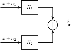
Fusion of two noisy sensors with Dynamics
  \begin{tikzpicture}
    \node[branch] (x) at (0, 0);
    \node[block, above right=1.5 and 0.5 of x](G1){$G_1$};
    \node[block, below right=1.5 and 0.5 of x](G2){$G_2$};
    \node[addb, right=1 of G1](add1){};
    \node[addb, right=1 of G2](add2){};
    \node[block, above=0.5 of add1](W1){$W_1$};
    \node[block, above=0.5 of add2](W2){$W_2$};
    \node[block, right=1 of add1](H1){$H_1$};
    \node[block, right=1 of add2](H2){$H_2$};
    \node[addb, right=6 of x](add){};

    \draw[] ($(x)+(-1, 0)$) node[above right]{$x$} -- (x);
    \draw[->] (x) |- (G1.west);
    \draw[->] (x) |- (G2.west);
    \draw[->] (G1.east) -- (add1.west);
    \draw[->] (G2.east) -- (add2.west);
    \draw[->] (W1.south) -- (add1.north);
    \draw[->] (W2.south) -- (add2.north);
    \draw[<-] (W1.north) -- ++(0, 0.8)node[below right]{$n_1$};
    \draw[<-] (W2.north) -- ++(0, 0.8)node[below right]{$n_2$};
    \draw[->] (add1.east) -- (H1.west);
    \draw[->] (add2.east) -- (H2.west);
    \draw[->] (H1) -| (add.north);
    \draw[->] (H2) -| (add.south);
    \draw[->] (add.east) -- ++(1, 0) node[above left]{$\hat{x}$};
  \end{tikzpicture}
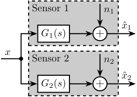
Fusion of two noisy sensors with Dynamics - Bis
  \begin{tikzpicture}
    \node[branch] (x) at (0, 0);
    \node[block, above right=0.5 and 0.5 of x](G1){$G_1$};
    \node[block, below right=0.5 and 0.5 of x](G2){$G_2$};
    \node[addb, right=1 of G1](add1){};
    \node[addb, right=1 of G2](add2){};
    \node[block, right=1 of add1](H1){$H_1$};
    \node[block, right=1 of add2](H2){$H_2$};
    \node[addb, right=6 of x](add){};

    \draw[] ($(x)+(-1, 0)$) node[above right]{$x$} -- (x);
    \draw[->] (x) |- (G1.west);
    \draw[->] (x) |- (G2.west);
    \draw[->] (G1.east) -- (add1.west);
    \draw[->] (G2.east) -- (add2.west);
    \draw[<-] (add1.north) -- ++(0, 0.8)node[below right]{$n_1$};
    \draw[<-] (add2.north) -- ++(0, 0.8)node[below right]{$n_2$};
    \draw[->] (add1.east) -- (H1.west);
    \draw[->] (add2.east) -- (H2.west);
    \draw[->] (H1) -| (add.north);
    \draw[->] (H2) -| (add.south);
    \draw[->] (add.east) -- ++(1, 0) node[above left]{$\hat{x}$};
  \end{tikzpicture}
Fusion of two sensors with mismatch dynamics
  <<tikz_default>>
  \begin{tikzpicture}
    \node[branch] (x) at (0, 0);
    \node[addb, above right=1 and 3.5 of x](add1){};
    \node[addb, below right=1 and 3.5 of x](add2){};
    \node[block, above left= of add1](delta1){$\Delta_1$};
    \node[block, above left= of add2](delta2){$\Delta_2$};
    \node[block, left= of delta1](W1){$W_1$};
    \node[block, left= of delta2](W2){$W_2$};
    \node[block, right= of add1](H1){$H_1$};
    \node[block, right= of add2](H2){$H_2$};
    \node[addb, right=5.5 of x](add){};

    \draw[] ($(x)+(-1, 0)$) node[above right]{$x$} -- (x);
    \draw[->] (x) |- (add1.west);
    \draw[->] (x) |- (add2.west);
    \draw[->] ($(add1-|W1.west)+(-0.5, 0)$)node[branch]{} |- (W1.west);
    \draw[->] ($(add2-|W2.west)+(-0.5, 0)$)node[branch]{} |- (W2.west);
    \draw[->] (W1.east) -- (delta1.west);
    \draw[->] (W2.east) -- (delta2.west);
    \draw[->] (delta1.east) -| (add1.north);
    \draw[->] (delta2.east) -| (add2.north);
    \draw[->] (add1.east) -- (H1.west);
    \draw[->] (add2.east) -- (H2.west);
    \draw[->] (H1.east) -| (add.north);
    \draw[->] (H2.east) -| (add.south);
    \draw[->] (add.east) -- ++(1, 0) node[above left]{$\hat{x}$};
  \end{tikzpicture}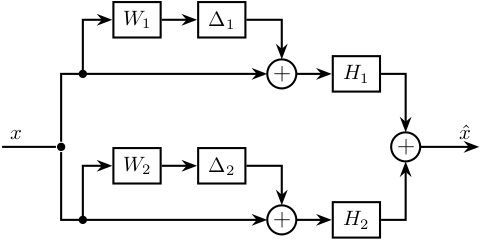
Uncertainty to Phase and Gain variation
  \begin{tikzpicture}
    \draw[->] (-0.5, 0)   -- (7, 0) node[below left]{Real};
    \draw[->] (0, -1) -- (0, 1) node[left]{Im};
    \node[branch] (1) at (5, 0){};
    \node[below] at (1){$1$};
    \node[circle, draw] (c) at (1)[minimum size=2cm]{};
    \draw[dashed] (0, 0) -- (tangent cs:node=c,point={(0, 0)},solution=2) -- node[midway, right]{$|H_i W_i|$} (1);
    \draw[dashed] (2, 0) arc (0:23:1) node[midway, right]{$\Delta \phi$};
    % \draw[dashed] (0, 0) -- (tangent cs:node=c,point={(0, 0)},solution=1) coordinate(cbot);
  \end{tikzpicture}
Generate Complementary Filters using Feedback Control Architecture
  \begin{tikzpicture}
    \node[addb={+}{}{}{}{-}] (addfb) at (0, 0){};
    \node[block, right=1 of addfb] (L){$L$};
    \node[addb={+}{}{}{}{}, right=1 of L] (adddy){};

    \draw[<-] (addfb.west) -- ++(-1, 0) node[above right]{$y_1$};
    \draw[->] (addfb.east) -- (L.west);
    \draw[->] (L.east) -- (adddy.west);
    \draw[->] (adddy.east) -- ++(1, 0) node[above left]{$y_s$};
    \draw[->] ($(adddy.east) + (0.5, 0)$) node[branch]{} -- ++(0, -1) -| (addfb.south);
    \draw[<-] (adddy.north) -- ++(0, 1) node[below right]{$y_2$};
  \end{tikzpicture}
H-Infinity Synthesis for Robust Sensor Fusion
  <<tikz_default>>
  \begin{tikzpicture}
     \node[block={4.0cm}{3.0cm}, dashed] (P) {};
     \node[above] at (P.north) {$P$};

     \coordinate[] (inputw)  at ($(P.south west)!0.8!(P.north west) + (-\cdist, 0)$);
     \coordinate[] (inputu)  at ($(P.south west)!0.4!(P.north west) + (-\cdist, 0)$);

     \coordinate[] (outputh) at ($(P.south east)!0.8!(P.north east) + ( \cdist, 0)$);
     \coordinate[] (outputl) at ($(P.south east)!0.4!(P.north east) + ( \cdist, 0)$);
     \coordinate[] (outputv) at ($(P.south east)!0.1!(P.north east) + ( \cdist, 0)$);

     \node[block, left=2*\cdist of outputl] (W1){$w_1$};
     \node[block, left=2*\cdist of outputh] (W2){$w_2$};
     \node[addb={+}{}{}{}{-}, left=of W2] (sub) {};

     \node[block, below=\cdist of P] (H1) {$H_1$};

     \draw[->] (inputw) node[above right]{$w$} -- (sub.west);
     \draw[->] (H1.west) -| ($(inputu)+(0.5*\cdist, 0)$) -- (W1.west);
     \draw[->] (inputu-|sub) node[branch]{} -- (sub.south);
     \draw[->] (sub.east) -- (W2.west);
     \draw[->] ($(inputw)+(2*\cdist, 0)$) node[branch]{} |- ($(outputv)+(-0.5*\cdist, 0)$) |- (H1.east);
     \draw[->] (W2.east) -- (outputh)node[above left]{$z_2$};
     \draw[->] (W1.east) -- (outputl)node[above left]{$z_1$};
  \end{tikzpicture}
Sensor fusion architecture with sensor dynamics uncertainty and noise
  <<tikz_default>>
  \begin{tikzpicture}
    \node[branch] (x) at (0, 0);
    \node[addb, above right=1.2 and 3.7 of x](add1){};
    \node[addb, below right=1.2 and 3.7 of x](add2){};
    \node[block, above left=0.2 and 0.1 of add1](delta1){$\Delta_1(s)$};
    \node[block, above left=0.2 and 0.1 of add2](delta2){$\Delta_2(s)$};
    \node[block, left=0.5 of delta1](W1){$w_1(s)$};
    \node[block, left=0.5 of delta2](W2){$w_2(s)$};
    \node[addb, right=0.5 of add1](addn1){};
    \node[addb, right=0.5 of add2](addn2){};
    \node[block, above=0.5 of addn1](N1) {$N_1(s)$};
    \node[block, above=0.5 of addn2](N2) {$N_2(s)$};
    \node[block, right=1.2 of addn1](H1){$H_1(s)$};
    \node[block, right=1.2 of addn2](H2){$H_2(s)$};
    \node[addb, right=7.5 of x](add){};

    \draw[] ($(x)+(-0.7, 0)$) node[above right]{$x$} -- (x.center);
    \draw[->] (x.center) |- (add1.west);
    \draw[->] (x.center) |- (add2.west);
    \draw[->] ($(add1-|W1.west)+(-0.5, 0)$)node[branch](S1){} |- (W1.west);
    \draw[->] ($(add2-|W2.west)+(-0.5, 0)$)node[branch](S2){} |- (W2.west);
    \draw[->] (W1.east) -- (delta1.west);
    \draw[->] (W2.east) -- (delta2.west);
    \draw[->] (delta1.east) -| (add1.north);
    \draw[->] (delta2.east) -| (add2.north);
    \draw[->] (add1.east) -- (addn1.west);
    \draw[->] (add2.east) -- (addn2.west);
    \draw[->] (addn1.east) -- (H1.west)node[above left]{$\hat{x}_1$};
    \draw[->] (addn2.east) -- (H2.west)node[above left]{$\hat{x}_2$};
    \draw[->] ($(N1.north)+(0,0.7)$) node[below right](n1){$\tilde{n}_1$} -- (N1.north);
    \draw[->] ($(N2.north)+(0,0.7)$) node[below right](n2){$\tilde{n}_2$} -- (N2.north);
    \draw[->] (N1.south) -- (addn1.north)node[above right]{$n_1$};
    \draw[->] (N2.south) -- (addn2.north)node[above right]{$n_2$};
    \draw[->] (H1.east) -| (add.north);
    \draw[->] (H2.east) -| (add.south);
    \draw[->] (add.east) -- ++(0.7, 0) node[above left]{$\hat{x}$};

    \begin{scope}[on background layer]
      \node[fit={($(add2.south-|x)+(-0.2, -0.4)$) ($(n1.north-|add.east)+(0.2, 0.3)$)}, fill=black!10!white, draw, dashed, inner sep=0pt] (supersensor) {};
      \node[below left] at (supersensor.north east) {Super Sensor};
      \node[block, fit={($(S1|-add1.south)+(-0.2, -0.2)$) ($(n1.north-|N1.east)+(0.2, 0.1)$)}, fill=black!20!white, dashed, inner sep=0pt] (sensor1) {};
      \node[below right] at (sensor1.north west) {Sensor 1};
      \node[block, fit={($(S2|-add2.south)+(-0.2, -0.2)$) ($(n2.north-|N2.east)+(0.2, 0.1)$)}, fill=black!20!white, dashed, inner sep=0pt] (sensor2) {};
      \node[below right] at (sensor2.north west) {Sensor 2};
    \end{scope}
  \end{tikzpicture}
Equivalent super sensor
  <<tikz_default>>
  \begin{tikzpicture}
    \node[branch] (x) at (0, 0);
    \node[block, above right=0.6 and 0.4 of x](Wss){$w_{ss}(s)$};
    \node[block, right=0.5 of Wss](delta){$\Delta(s)$};
    \node[addb](add) at ($(delta.east|-x) + (0.5, 0)$){};
    \node[addb, right=0.5 of add](addn){};
    \node[block](Nss) at (delta-|addn) {$N_{ss}(s)$};

    \draw[] ($(x)+(-0.7, 0)$) node[above right]{$x$} -- (add.west);
    \draw[->] (x.center) |- (Wss);
    \draw[->] (Wss.east) -- (delta.west);
    \draw[->] (delta.east) -| (add.north);
    \draw[->] (add.east) -- (addn.west);
    \draw[->] ($(Nss.north)+(0,0.7)$) node[below right](nss){$\hat{n}$} -- (Nss.north);
    \draw[->] (Nss.south) -- (addn.north) node[above right]{$n$};
    \draw[->] (addn.east) -- ++(1.1, 0) node[above left]{$\hat{x}$};

    \begin{scope}[on background layer]
      \node[fit={($(add.south-|x)+(-0.2, -0.2)$) ($(Nss.east|-nss.north)+(0.2, 0.2)$)}, fill=black!10!white, draw, dashed, inner sep=0pt] (supersensor) {};
      \node[below right] at (supersensor.north west) {Super Sensor};
    \end{scope}
  \end{tikzpicture}
One sensor with noise
  <<tikz_default>>
  \begin{tikzpicture}
    \node[block] (G) at (0, 0) {$G(s)$};
    \node[addb, right=0.8 of G] (add) {};

    \draw[->] ($(G.west) + (-0.8, 0)$)node[above right]{$x$} -- (G.west);
    \draw[->] (G.east) -- (add.west);
    \draw[->] ($(add.north) + (0, 0.8)$)node[below right](n){$n$} -- (add.north);
    \draw[->] (add.east) -- ++(0.8, 0) node[above left]{$\hat{x}$};

    \begin{scope}[on background layer]
      \node[fit={($(G.south west)+(-0.3, -0.1)$) ($(n.north east)+(0.0, 0.1)$)}, fill=black!20!white, draw, dashed, inner sep=0pt] (sensor) {};
      \node[below right] at (sensor.north west) {Sensor};
    \end{scope}
  \end{tikzpicture}
One sensor with normalized noise
  <<tikz_default>>
  \begin{tikzpicture}
    \node[block] (G) at (0, 0) {$G(s)$};
    \node[addb, right=0.8 of G] (add) {};
    \node[block, above=0.6 of add] (N) {$N(s)$};

    \draw[->] ($(G.west) + (-0.8, 0)$)node[above right]{$x$} -- (G.west);
    \draw[->] (G.east) -- (add.west);
    \draw[->] ($(N.north) + (0, 0.8)$)node[below right](ntilde){$\tilde{n}$} -- (N.north);
    \draw[->] (N.south) -- (add.north)node[above right](n){$n$};
    \draw[->] (add.east) -- ++(1.0, 0) node[above left]{$\hat{x}$};

    \begin{scope}[on background layer]
      \node[fit={($(G.south west)+(-0.3, -0.2)$) ($(ntilde.north-|N.east)+(0.2, 0.1)$)}, fill=black!20!white, draw, dashed, inner sep=0pt] (sensor) {};
      \node[below right] at (sensor.north west) {Sensor};
    \end{scope}
  \end{tikzpicture}
One sensor with dynamic uncertainty
  <<tikz_default>>
  \begin{tikzpicture}
    \node[branch] (x) at (0, 0) {};
    \node[block, above right=0.4 and 0.4 of x](W){$w(s)$};
    \node[block, right=0.4 of W](delta){$\Delta(s)$};
    \node[addb](add) at ($(delta.east|-x) + (0.4, 0)$) {};
    \node[block, right=0.5 of add](G){$G(s)$};

    \draw[->] ($(x.west) + (-0.8, 0)$)node[above right]{$x$} -- (add.west);
    \draw[->] (x.center) |- (W.west);
    \draw[->] (W.east) -- (delta.west);
    \draw[->] (delta.east) -| (add.north);
    \draw[->] (add.east) -- (G.west);
    \draw[->] (G.east) -- ++(0.8, 0) node[above left]{$\hat{x}$};

    \begin{scope}[on background layer]
      \node[fit={($(x.west|-G.south)+(-0.2, -0.2)$) ($(delta.north-|G.east)+(0.2, 0.2)$)}, fill=black!20!white, draw, dashed, inner sep=0pt] (sensor) {};
      \node[below left] at (sensor.north east) {Sensor};
    \end{scope}
  \end{tikzpicture}
One sensor with dynamic uncertainty and noise
  <<tikz_default>>
  \begin{tikzpicture}
    \node[branch] (x) at (0, 0) {};
    \node[block, above right=0.4 and 0.4 of x](W){$w(s)$};
    \node[block, right=0.4 of W](delta){$\Delta(s)$};
    \node[addb](add) at ($(delta.east|-x) + (0.4, 0)$) {};
    \node[block, right=0.5 of add](G){$G(s)$};
    \node[addb, right=0.5 of G] (addn) {};

    \draw[->] ($(x.west) + (-0.8, 0)$)node[above right]{$x$} -- (add.west);
    \draw[->] (x.center) |- (W.west);
    \draw[->] (W.east) -- (delta.west);
    \draw[->] (delta.east) -| (add.north);
    \draw[->] (add.east) -- (G.west);
    \draw[->] (G.east) -- (addn.west);
    \draw[->] ($(addn.north)+(0, 0.8)$) node[below right]{$n$} -- (addn.north);
    \draw[->] (addn.east) -- ++(0.8, 0) node[above left]{$\hat{x}$};

    \begin{scope}[on background layer]
      \node[fit={($(x.west|-G.south)+(-0.2, -0.2)$) ($(delta.north-|addn.east)+(0.2, 0.2)$)}, fill=black!20!white, draw, dashed, inner sep=0pt] (sensor) {};
      \node[above right] at (sensor.south west) {Sensor};
    \end{scope}
  \end{tikzpicture}
Huddle Test
  <<tikz_default>>

  \begin{tikzpicture}
    \node[branch] (x) at (0, 0);
    \node[block, above right=0.5 and 0.5 of x](G1){$G_1(s)$};
    \node[block, below right=0.5 and 0.5 of x](G2){$G_2(s)$};
    \node[addb, right=0.8 of G1](add1){};
    \node[addb, right=0.8 of G2](add2){};

    \draw[] ($(x)+(-0.7, 0)$) node[above right]{$x$} -- (x.center);
    \draw[->] (x.center) |- (G1.west);
    \draw[->] (x.center) |- (G2.west);
    \draw[->] (G1.east) -- (add1.west);
    \draw[->] (G2.east) -- (add2.west);
    \draw[<-] (add1.north) -- ++(0, 0.8)node[below right](n1){$n_1$};
    \draw[<-] (add2.north) -- ++(0, 0.8)node[below right](n2){$n_2$};
    \draw[->] (add1.east) -- ++(1, 0)node[above left]{$\hat{x}_1$};
    \draw[->] (add2.east) -- ++(1, 0)node[above left]{$\hat{x}_2$};

    \begin{scope}[on background layer]
      % \node[fit={($(G2.south-|x)+(-0.2, -0.3)$) ($(n1.north east-|add.east)+(0.2, 0.3)$)}, fill=black!10!white, draw, dashed, inner sep=0pt] (supersensor) {};
      % \node[below left] at (supersensor.north east) {Super Sensor};

      \node[fit={($(G1.south west)+(-0.3, -0.1)$) ($(n1.north east)+(0.0, 0.1)$)}, fill=black!20!white, draw, dashed, inner sep=0pt] (sensor1) {};
      \node[below right] at (sensor1.north west) {Sensor 1};
      \node[fit={($(G2.south west)+(-0.3, -0.1)$) ($(n2.north east)+(0.0, 0.1)$)}, fill=black!20!white, draw, dashed, inner sep=0pt] (sensor2) {};
      \node[below right] at (sensor2.north west) {Sensor 2};
    \end{scope}
  \end{tikzpicture}