43 KiB
On the Design of Complementary Filters for Control - Computation with Matlab
- Introduction
- Optimal Sensor Fusion for noise characteristics
- Robustness to sensor dynamics uncertainty
- Complementary filters using analytical formula
- H-Infinity synthesis of complementary filters
- Feedback Control Architecture to generate Complementary Filters
- Bibliography
Introduction ignore
In this document, the design of complementary filters is studied.
One use of complementary filter is described below:
The basic idea of a complementary filter involves taking two or more sensors, filtering out unreliable frequencies for each sensor, and combining the filtered outputs to get a better estimate throughout the entire bandwidth of the system. To achieve this, the sensors included in the filter should complement one another by performing better over specific parts of the system bandwidth.
- in section sec:optimal_comp_filters, the optimal design of the complementary filters in order to obtain the lowest resulting "super sensor" noise is studied
When blending two sensors using complementary filters with unknown dynamics, phase lag may be introduced that renders the close-loop system unstable.
- in section sec:comp_filter_robustness, the blending robustness to sensor dynamic uncertainty is studied.
Then, three design methods for generating two complementary filters are proposed:
- in section sec:comp_filters_analytical, analytical formulas are proposed
- in section sec:h_inf_synthesis_complementary_filters, the $\mathcal{H}_\infty$ synthesis is used
- in section sec:feedback_generate_comp_filters, the classical feedback architecture is used
Optimal Sensor Fusion for noise characteristics
<<sec:optimal_comp_filters>>
Introduction ignore
The idea is to combine sensors that works in different frequency range using complementary filters.
Doing so, one "super sensor" is obtained that can have better noise characteristics than the individual sensors over a large frequency range.
The complementary filters have to be designed in order to minimize the effect noise of each sensor on the super sensor noise.
ZIP file containing the data and matlab files ignore
All the files (data and Matlab scripts) are accessible here.
Architecture
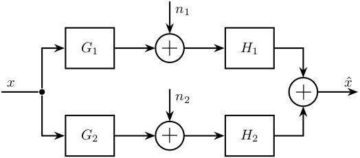
Let's consider the sensor fusion architecture shown on figure fig:fusion_two_noisy_sensors_with_dyn where two sensors 1 and 2 are measuring the same quantity $x$ with different noise characteristics determined by $W_1$ and $W_2$.
$n_1$ and $n_2$ are white noise (constant power spectral density over all frequencies).
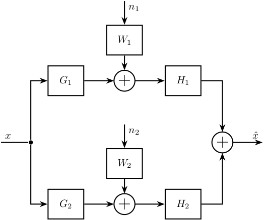
We consider that the two sensor dynamics $G_1$ and $G_2$ are ideal ($G_1 = G_2 = 1$). We obtain the architecture of figure fig:fusion_two_noisy_sensors.
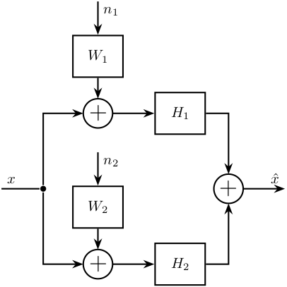
$H_1$ and $H_2$ are complementary filters ($H_1 + H_2 = 1$). The goal is to design $H_1$ and $H_2$ such that the effect of the noise sources $n_1$ and $n_2$ has the smallest possible effect on the estimation $\hat{x}$.
We have that the Power Spectral Density (PSD) of $\hat{x}$ is: \[ \Gamma_{\hat{x}} = |H_1 W_1|^2 \Gamma_{n_1} + |H_2 W_2|^2 \Gamma_{n_2} \]
And the goal is the minimize the Root Mean Square (RMS) value of $\hat{x}$: \[ \sigma_{\hat{x}} = \sqrt{\int_0^\infty \Gamma_{\hat{x}}(\omega) d\omega} \]
As $n_1$ and $n_2$ are white noise: $\Gamma_{n_1} = \Gamma_{n_2} = 1$ and we have: \[ \sigma_{\hat{x}} = \sqrt{\int_0^\infty |H_1 W_1|^2(\omega) + |H_2 W_2|^2(\omega) d\omega} = \left\| \begin{matrix} H_1 W_1 \\ H_2 W_2 \end{matrix} \right\|_2 \]
Thus, the goal is to design $H_1$ and $H_2$ such that $H_1 + H_2 = 1$ and such that $\left\| \begin{matrix} H_1 W_1 \\ H_2 W_2 \end{matrix} \right\|_2$ is minimized.
For that, we will use the $\mathcal{H}_2$ Synthesis.
Noise of the sensors
Let's define the noise characteristics of the two sensors by choosing $W_1$ and $W_2$:
- Sensor 1 characterized by $W_1$ has low noise at low frequency (for instance a geophone)
- Sensor 2 characterized by $W_2$ has low noise at high frequency (for instance an accelerometer)
  omegac = 100*2*pi; G0 = 1e-5; Ginf = 1e-4;
  W1 = (Ginf*s/omegac + G0)/(s/omegac + 1)/(1 + s/2/pi/4000);

  omegac = 1*2*pi; G0 = 1e-3; Ginf = 1e-8;
W2 = ((sqrt(Ginf)*s/omegac + sqrt(G0))/(s/omegac + 1))^2/(1 + s/2/pi/4000)^2; <<plt-matlab>>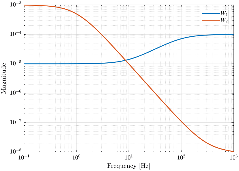
H-Two Synthesis
We use the generalized plant architecture shown on figure fig:h_infinity_optimal_comp_filters.
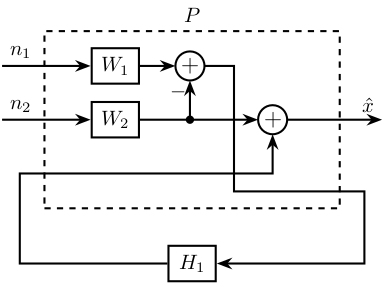
The transfer function from $[n_1, n_2]$ to $\hat{x}$ is: \[ \begin{bmatrix} W_1 H_1 \\ W_2 (1 - H_1) \end{bmatrix} \] If we define $H_2 = 1 - H_1$, we obtain: \[ \begin{bmatrix} W_1 H_1 \\ W_2 H_2 \end{bmatrix} \]
Thus, if we minimize the $\mathcal{H}_2$ norm of this transfer function, we minimize the RMS value of $\hat{x}$.
We define the generalized plant $P$ on matlab as shown on figure fig:h_infinity_optimal_comp_filters.
  P = [0   W2  1;
       W1 -W2  0];
And we do the $\mathcal{H}_2$ synthesis using the h2syn command.
[H1, ~, gamma] = h2syn(P, 1, 1);
What is minimized is norm([W1*H1,W2*H2], 2).
Finally, we define $H_2 = 1 - H_1$.
H2 = 1 - H1;Analysis
The complementary filters obtained are shown on figure fig:htwo_comp_filters. The PSD of the fig:psd_sensors_htwo_synthesis. Finally, the RMS value of $\hat{x}$ is shown on table tab:rms_results. The optimal sensor fusion has permitted to reduced the RMS value of the estimation error by a factor 8 compare to when using only one sensor.
<<plt-matlab>>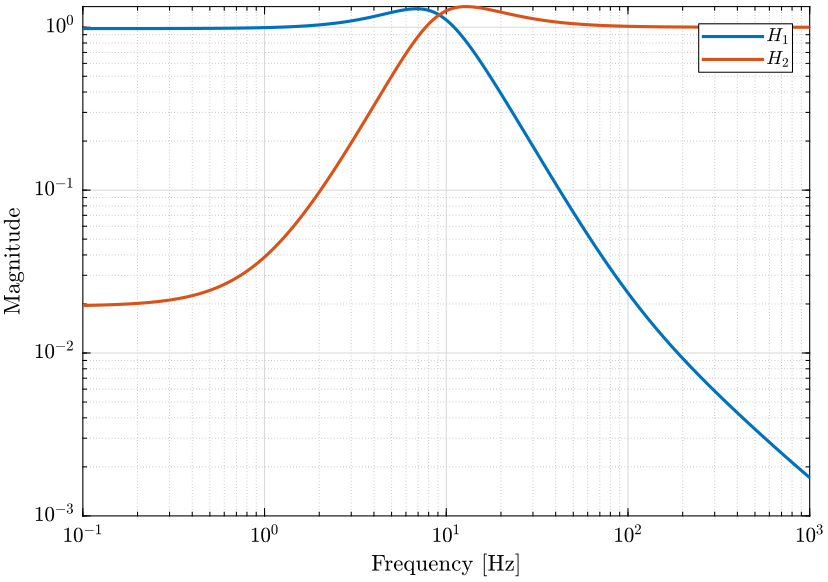
<<plt-matlab>>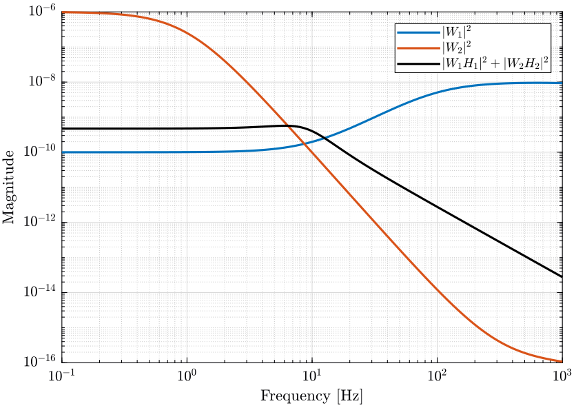
| rms value | |
|---|---|
| Sensor 1 | 1.1e-02 |
| Sensor 2 | 1.3e-03 |
| Optimal Sensor Fusion | 1.5e-04 |
Robustness to sensor dynamics uncertainty
<<sec:comp_filter_robustness>>
Introduction ignore
Let's first consider ideal sensors where $G_1 = 1$ and $G_2 = 1$ (figure fig:fusion_two_noisy_sensors_with_dyn_bis).
We then have:
\begin{align*} \hat{x} &= (x + n_1) H_1 + (x + n_2) H_2 \\ &= x + n_1 H_1 + n_2 H_2 \end{align*}So the estimation error is \[ \delta_x = \hat{x} - x = n_1 H_1 + n_2 H_2 \]
And we see that the complementary filters are only shaping the noise and that they do not impact the transfer function from $x$ to $\hat{x}$ that is in the feedback path.
ZIP file containing the data and matlab files ignore
All the files (data and Matlab scripts) are accessible here.
Unknown sensor dynamics dynamics
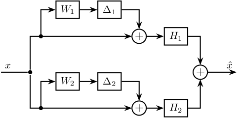
In practical systems, the sensor dynamics has always some level of uncertainty. Let's represent that with multiplicative input uncertainty as shown on figure fig:fusion_gain_mismatch.
We have:
\begin{align*} \frac{\hat{x}}{x} &= (1 + W_1 \Delta_1) H_1 + (1 + W_2 \Delta_2) H_2 \\ &= 1 + W_1 H_1 \Delta_1 + W_2 H_2 \Delta_2 \end{align*}With $\Delta_i$ is any transfer function satisfying $\| \Delta_i \|_\infty < 1$.
We see that as soon as we have some uncertainty in the sensor dynamics, we have that the complementary filters have some effect on the transfer function from $x$ to $\hat{x}$.
We want that the super sensor transfer function has a gain of 1 and no phase variation over all the frequencies: \[ \frac{\hat{x}}{x} \approx 1 \]
Thus, we want that
\begin{align*} & |W_1 H_1 \Delta_1 + W_2 H_2 \Delta_2| < \epsilon \quad \forall \omega, \forall \Delta_i, \|\Delta_i\|_\infty < 1 \\ \Longleftrightarrow & |W_1 H_1| + |W_2 H_2| < \epsilon \quad \forall \omega \end{align*}Which is approximately the same as requiring \[ \left\| \begin{matrix} W_1 H_1 \\ W_2 H_2 \end{matrix} \right\|_\infty < \epsilon \]
How small should we choose $\epsilon$?
The uncertainty set of the transfer function from $\hat{x}$ to $x$ is bounded in the complex plane by a circle centered on 1 and with a radius equal to $\epsilon$ (figure fig:uncertainty_gain_phase_variation).
We then have that the angle introduced by the super sensor is bounded by $\arcsin(\epsilon)$: \[ \angle \frac{\hat{x}}{x} \le \arcsin (\epsilon) \quad \forall \omega \]

Thus, we choose should choose $\epsilon$ so that the maximum phase uncertainty introduced by the sensors is of an acceptable value.
Design the complementary filters in order to limit the phase and gain uncertainty of the super sensor
Let's say the two sensors dynamics $H_1$ and $H_2$ have been identified with the associated uncertainty weights $W_1$ and $W_2$.
If we want to have a maximum phase introduced by the sensors of 20 degrees, we have to design $H_1$ and $H_2$ such that:
\begin{align*} & arcsin(|H_1 W_1| + |H_2 W_2|) < 20 \text{ deg} \\ \Longleftrightarrow & |H_1 W_1| + |H_2 W_2| < 0.34 \end{align*}We can do that with the $\mathcal{H}_\infty$ synthesis by setting upper bounds on the complementary filters using weights that corresponds to the sensor dynamics uncertainty.
For simplicity, let's suppose $W_1(s) = W_2(s) = 0.1$ ($10\%$ uncertainty in the sensor gain). \[ |H_1 W_1| + |H_2 W_2| < 3.4 \]
Thus, by limiting the norm of the complementary filters, we can limit the maximum unwanted phase introduced by the uncertainty on the sensors dynamics.
This is of primary importance in order to ensure the stability of the feedback loop using the super sensor signal.
First Basic Example with gain mismatch
Let's consider two ideal sensors except one sensor has not an expected gain of one but a gain of $0.6$.
  G1 = 1;
  G2 = 0.6;
Let's design two complementary filters as shown on figure fig:comp_filters_robustness_test. The complementary filters shown in blue does not present a bump as the red ones but provides less sensor separation at high and low frequencies.
<<plt-matlab>>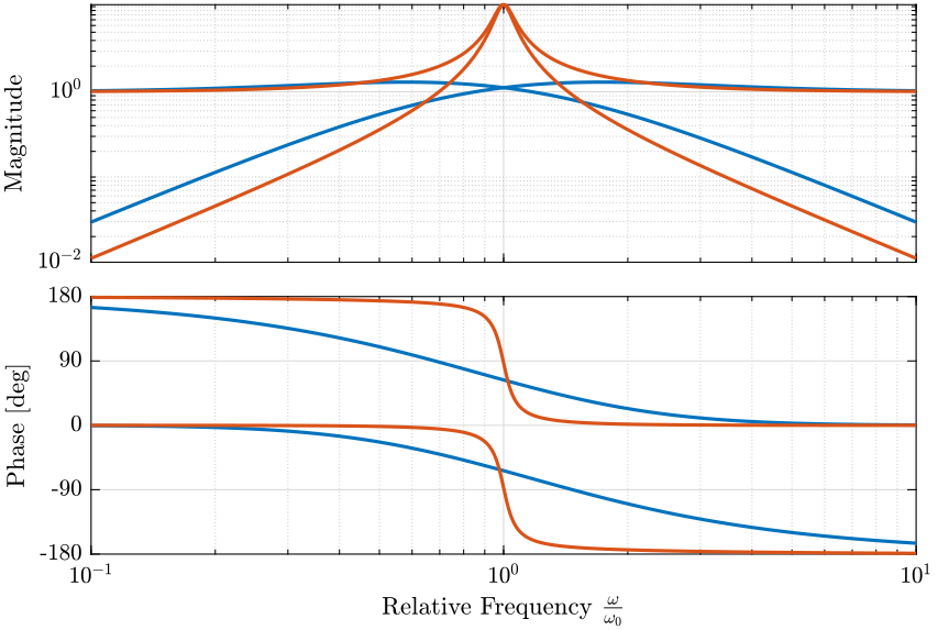
We then compute the bode plot of the super sensor transfer function $H_1*G_1 + H_2*G_2$ for both complementary filters pair (figure fig:tf_super_sensor_comp).
We see that the blue complementary filters with a lower maximum norm permits to limit the phase lag introduced by the gain mismatch.
<<plt-matlab>>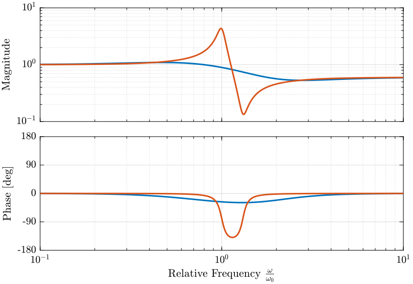
TODO More Complete example with model uncertainty
Complementary filters using analytical formula
<<sec:comp_filters_analytical>>
Introduction ignore
ZIP file containing the data and matlab files ignore
All the files (data and Matlab scripts) are accessible here.
Analytical 1st order complementary filters
First order complementary filters are defined with following equations:
\begin{align} H_L(s) = \frac{1}{1 + \frac{s}{\omega_0}}\\ H_H(s) = \frac{\frac{s}{\omega_0}}{1 + \frac{s}{\omega_0}} \end{align}Their bode plot is shown figure fig:comp_filter_1st_order.
  w0 = 2*pi; % [rad/s]

  Hh1 = (s/w0)/((s/w0)+1);
Hl1 = 1/((s/w0)+1); <<plt-matlab>>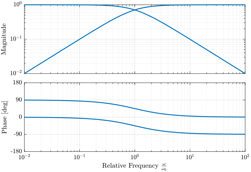
Second Order Complementary Filters
We here use analytical formula for the complementary filters $H_L$ and $H_H$.
The first two formulas that are used to generate complementary filters are:
\begin{align*} H_L(s) &= \frac{(1+\alpha) (\frac{s}{\omega_0})+1}{\left((\frac{s}{\omega_0})+1\right) \left((\frac{s}{\omega_0})^2 + \alpha (\frac{s}{\omega_0}) + 1\right)}\\ H_H(s) &= \frac{(\frac{s}{\omega_0})^2 \left((\frac{s}{\omega_0})+1+\alpha\right)}{\left((\frac{s}{\omega_0})+1\right) \left((\frac{s}{\omega_0})^2 + \alpha (\frac{s}{\omega_0}) + 1\right)} \end{align*}where:
- $\omega_0$ is the blending frequency in rad/s.
-
$\alpha$ is used to change the shape of the filters:
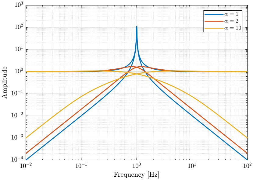
- Small values for $\alpha$ will produce high magnitude of the filters $|H_L(j\omega)|$ and $|H_H(j\omega)|$ near $\omega_0$ but smaller value for $|H_L(j\omega)|$ above $\approx 1.5 \omega_0$ and for $|H_H(j\omega)|$ below $\approx 0.7 \omega_0$
- A large $\alpha$ will do the opposite
This is illustrated on figure fig:comp_filters_param_alpha. The slope of those filters at high and low frequencies is $-2$ and $2$ respectively for $H_L$ and $H_H$.
<<plt-matlab>>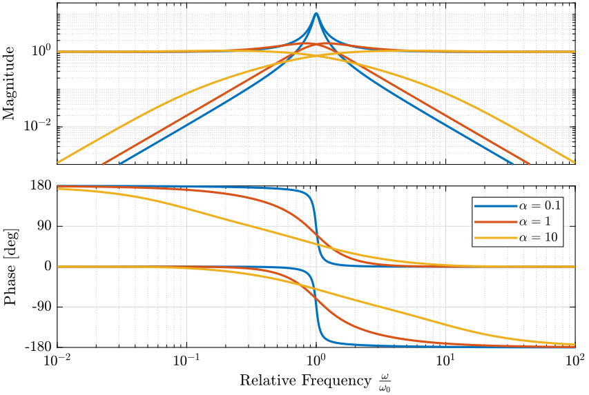
We now study the maximum norm of the filters function of the parameter $\alpha$. As we saw that the maximum norm of the filters is important for the robust merging of filters.
  figure;
  plot(alphas, infnorms)
  set(gca, 'xscale', 'log'); set(gca, 'yscale', 'log');
xlabel('$\alpha$'); ylabel('$\|H_1\|_\infty$'); <<plt-matlab>>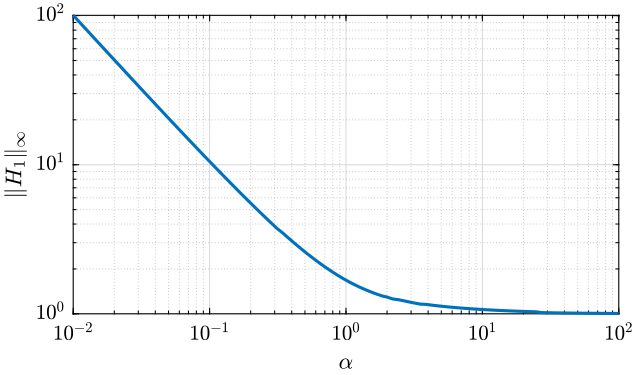
Third Order Complementary Filters
The following formula gives complementary filters with slopes of $-3$ and $3$:
\begin{align*} H_L(s) &= \frac{\left(1+(\alpha+1)(\beta+1)\right) (\frac{s}{\omega_0})^2 + (1+\alpha+\beta)(\frac{s}{\omega_0}) + 1}{\left(\frac{s}{\omega_0} + 1\right) \left( (\frac{s}{\omega_0})^2 + \alpha (\frac{s}{\omega_0}) + 1 \right) \left( (\frac{s}{\omega_0})^2 + \beta (\frac{s}{\omega_0}) + 1 \right)}\\ H_H(s) &= \frac{(\frac{s}{\omega_0})^3 \left( (\frac{s}{\omega_0})^2 + (1+\alpha+\beta) (\frac{s}{\omega_0}) + (1+(\alpha+1)(\beta+1)) \right)}{\left(\frac{s}{\omega_0} + 1\right) \left( (\frac{s}{\omega_0})^2 + \alpha (\frac{s}{\omega_0}) + 1 \right) \left( (\frac{s}{\omega_0})^2 + \beta (\frac{s}{\omega_0}) + 1 \right)} \end{align*}The parameters are:
- $\omega_0$ is the blending frequency in rad/s
- $\alpha$ and $\beta$ that are used to change the shape of the filters similarly to the parameter $\alpha$ for the second order complementary filters
The filters are defined below and the result is shown on figure fig:complementary_filters_third_order.
  alpha = 1;
  beta = 10;
  w0 = 2*pi*14;

  Hh3_ana = (s/w0)^3 * ((s/w0)^2 + (1+alpha+beta)*(s/w0) + (1+(alpha+1)*(beta+1)))/((s/w0 + 1)*((s/w0)^2+alpha*(s/w0)+1)*((s/w0)^2+beta*(s/w0)+1));
Hl3_ana = ((1+(alpha+1)*(beta+1))*(s/w0)^2 + (1+alpha+beta)*(s/w0) + 1)/((s/w0 + 1)*((s/w0)^2+alpha*(s/w0)+1)*((s/w0)^2+beta*(s/w0)+1)); <<plt-matlab>>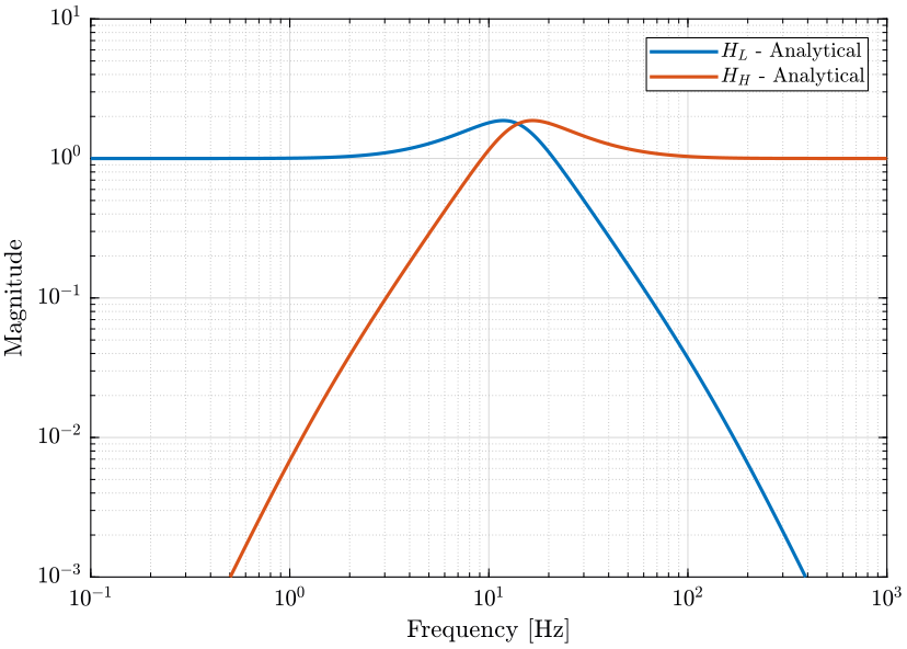
H-Infinity synthesis of complementary filters
<<sec:h_inf_synthesis_complementary_filters>>
Introduction ignore
ZIP file containing the data and matlab files ignore
All the files (data and Matlab scripts) are accessible here.
Synthesis Architecture
We here synthesize the complementary filters using the $\mathcal{H}_\infty$ synthesis. The goal is to specify upper bounds on the norms of $H_L$ and $H_H$ while ensuring their complementary property ($H_L + H_H = 1$).
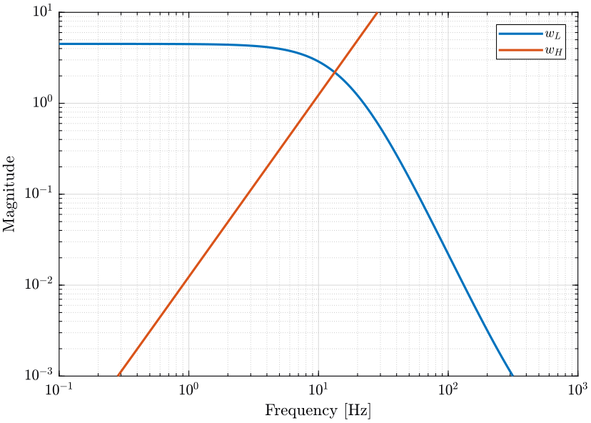
In order to do so, we use the generalized plant shown on figure fig:sf_hinf_filters_plant_b where $w_L$ and $w_H$ weighting transfer functions that will be used to shape $H_L$ and $H_H$ respectively.
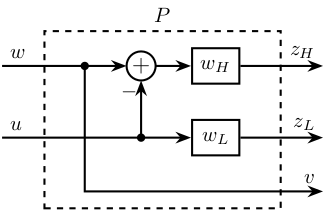
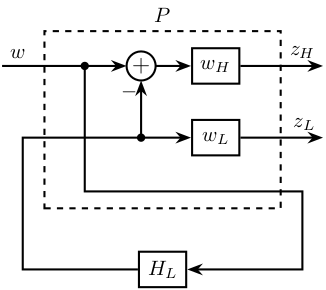
The $\mathcal{H}_\infty$ synthesis applied on this generalized plant will give a transfer function $H_L$ (figure fig:sf_hinf_filters_b) such that the $\mathcal{H}_\infty$ norm of the transfer function from $w$ to $[z_H,\ z_L]$ is less than one: \[ \left\| \begin{array}{c} H_L w_L \\ (1 - H_L) w_H \end{array} \right\|_\infty < 1 \]
Thus, if the above condition is verified, we can define $H_H = 1 - H_L$ and we have that: \[ \left\| \begin{array}{c} H_L w_L \\ H_H w_H \end{array} \right\|_\infty < 1 \] Which is almost (with an maximum error of $\sqrt{2}$) equivalent to:
\begin{align*} |H_L| &< \frac{1}{|w_L|}, \quad \forall \omega \\ |H_H| &< \frac{1}{|w_H|}, \quad \forall \omega \end{align*}We then see that $w_L$ and $w_H$ can be used to shape both $H_L$ and $H_H$ while ensuring (by definition of $H_H = 1 - H_L$) their complementary property.
Weights
H-Infinity Synthesis
We define the generalized plant $P$ on matlab.
  P = [0   wL;
       wH -wH;
       1   0];
And we do the $\mathcal{H}_\infty$ synthesis using the hinfsyn command.
[Hl_hinf, ~, gamma, ~] = hinfsyn(P, 1, 1,'TOLGAM', 0.001, 'METHOD', 'ric', 'DISPLAY', 'on');[Hl_hinf, ~, gamma, ~] = hinfsyn(P, 1, 1,'TOLGAM', 0.001, 'METHOD', 'ric', 'DISPLAY', 'on');
Test bounds: 0.0000 < gamma <= 1.7285
gamma hamx_eig xinf_eig hamy_eig yinf_eig nrho_xy p/f
1.729 4.1e+01 8.4e-12 1.8e-01 0.0e+00 0.0000 p
0.864 3.9e+01 -5.8e-02# 1.8e-01 0.0e+00 0.0000 f
1.296 4.0e+01 8.4e-12 1.8e-01 0.0e+00 0.0000 p
1.080 4.0e+01 8.5e-12 1.8e-01 0.0e+00 0.0000 p
0.972 3.9e+01 -4.2e-01# 1.8e-01 0.0e+00 0.0000 f
1.026 4.0e+01 8.5e-12 1.8e-01 0.0e+00 0.0000 p
0.999 3.9e+01 8.5e-12 1.8e-01 0.0e+00 0.0000 p
0.986 3.9e+01 -1.2e+00# 1.8e-01 0.0e+00 0.0000 f
0.993 3.9e+01 -8.2e+00# 1.8e-01 0.0e+00 0.0000 f
0.996 3.9e+01 8.5e-12 1.8e-01 0.0e+00 0.0000 p
0.994 3.9e+01 8.5e-12 1.8e-01 0.0e+00 0.0000 p
0.993 3.9e+01 -3.2e+01# 1.8e-01 0.0e+00 0.0000 f
Gamma value achieved: 0.9942
We then define the high pass filter $H_H = 1 - H_L$. The bode plot of both $H_L$ and $H_H$ is shown on figure fig:hinf_filters_results.
Hh_hinf = 1 - Hl_hinf;Obtained Complementary Filters
The obtained complementary filters are shown on figure fig:hinf_filters_results.
<<plt-matlab>>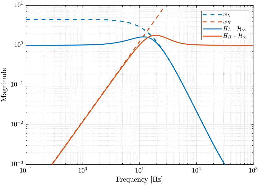
Feedback Control Architecture to generate Complementary Filters
<<sec:feedback_generate_comp_filters>>
Introduction ignore
The idea is here to use the fact that in a classical feedback architecture, $S + T = 1$, in order to design complementary filters.
Thus, all the tools that has been developed for classical feedback control can be used for complementary filter design.
ZIP file containing the data and matlab files ignore
All the files (data and Matlab scripts) are accessible here.
Architecture
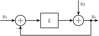
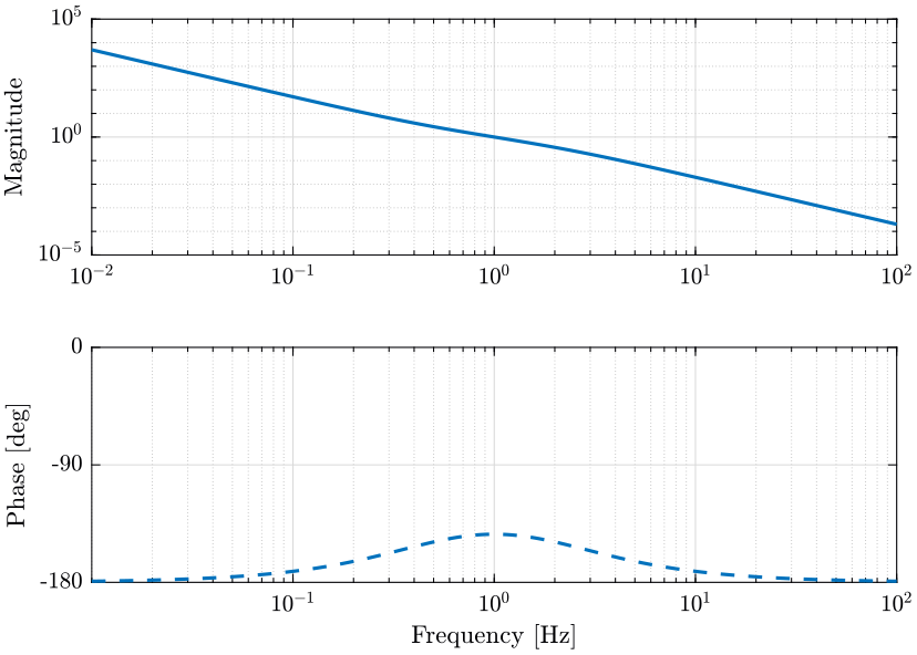
We have: \[ y = \underbrace{\frac{L}{L + 1}}_{H_L} y_1 + \underbrace{\frac{1}{L + 1}}_{H_H} y_2 \] with $H_L + H_H = 1$.
The only thing to design is $L$ such that the complementary filters are stable with the wanted shape.
A simple choice is: \[ L = \left(\frac{\omega_c}{s}\right)^2 \frac{\frac{s}{\omega_c / \alpha} + 1}{\frac{s}{\omega_c} + \alpha} \]
Which contains two integrator and a lead. $\omega_c$ is used to tune the crossover frequency and $\alpha$ the trade-off "bump" around blending frequency and filtering away from blending frequency.
Loop Gain Design
Bibliography ignore
bibliographystyle:unsrt bibliography:ref.bib
