148 KiB
Robust and Optimal Sensor Fusion - Matlab Computation
- Introduction
- Sensor Description
- First Order Complementary Filters
- Optimal Super Sensor Noise: $\mathcal{H}_2$ Synthesis with Acc and Pos
- Robust Sensor Fusion: $\mathcal{H}_\infty$ Synthesis with Acc and Pos
- Introduction
- ZIP file containing the data and matlab files
- Super Sensor Dynamical Uncertainty
- Synthesis objective
- Requirements as an $\mathcal{H}_\infty$ norm
- Weighting Function used to bound the super sensor uncertainty
- $\mathcal{H}_\infty$ Synthesis
- Super sensor uncertainty
- Super sensor noise
- Conclusion
- Optimal and Robust Sensor Fusion: Mixed $\mathcal{H}_2/\mathcal{H}_\infty$ Synthesis with Acc and Pos
- ZIP file containing the data and matlab files
- Mixed $\mathcal{H}_2$ / $\mathcal{H}_\infty$ Synthesis - Introduction
- Noise characteristics and Uncertainty of the individual sensors
- Weighting Functions on the uncertainty of the super sensor
- Mixed $\mathcal{H}_2$ / $\mathcal{H}_\infty$ Synthesis
- Obtained Super Sensor's noise
- Obtained Super Sensor's Uncertainty
- Comparison Hinf H2 H2/Hinf
- Conclusion
- Functions
- Bibliography
Introduction ignore
In this document, the optimal and robust design of complementary filters is studied.
Two sensors are considered with both different noise characteristics and dynamical uncertainties represented by multiplicative input uncertainty.
- Section sec:optimal_comp_filters: the $\mathcal{H}_2$ synthesis is used to design complementary filters such that the RMS value of the super sensor's noise is minimized
- Section sec:comp_filter_robustness: the $\mathcal{H}_\infty$ synthesis is used to design complementary filters such that the super sensor's uncertainty is bonded to acceptable values
- Section sec:mixed_synthesis_sensor_fusion: the mixed $\mathcal{H}_2/\mathcal{H}_\infty$ synthesis is used to both limit the super sensor's uncertainty and to lower the RMS value of the super sensor's noise
Sensor Description
Introduction ignore
- Schematic of one sensor
Sensor Dynamics
Accelerometer:
  m_acc = 0.01; % Inertial Mass [kg]
  c_acc = 5;    % Damping [N/(m/s)]
  k_acc = 1e5;  % Stiffness [N/m]
  g_acc = 1e5;  % Gain [V/m]

  G1 = -g_acc*m_acc*s/(m_acc*s^2 + c_acc*s + k_acc); % Accelerometer Plant [V/(m/s)]
Interferometer/Capacitive Sensor:
  w_pos = 2*pi*2e3; % Measurement Banwdith [rad/s]
  g_pos = 1e4; % Gain [V/m]

  G2 = g_pos/s/(1 + s/w_pos); % Position Sensor Plant [V/(m/s)]
Sensor Noise
Noise in $[m/s/\sqrt{Hz}]$.
  omegac = 0.05*2*pi; G0 = 1e-1; Ginf = 1e-6;
  N1 = (Ginf*s/omegac + G0)/(s/omegac + 1)/(1 + s/2/pi/1e4);

  omegac = 1000*2*pi; G0 = 1e-6; Ginf = 1e-3;
  N2 = (Ginf*s/omegac + G0)/(s/omegac + 1)/(1 + s/2/pi/1e4);
Sensor Model Uncertainty
The model uncertainty is described by multiplicative uncertainty.
  W1 = createWeight('n', 2, 'w0', 2*pi*3,   'G0', 2, 'G1', 0.1,     'Gc', 1) * ...
       createWeight('n', 2, 'w0', 2*pi*1e3, 'G0', 1, 'G1', 4/0.1, 'Gc', 1/0.1);

  W2 = createWeight('n', 2, 'w0', 2*pi*1e2, 'G0', 0.05, 'G1', 4, 'Gc', 1);
Save Model
save('./mat/model.mat', 'freqs', 'G1', 'G2', 'N2', 'N1', 'W2', 'W1');First Order Complementary Filters
Complementary Filters
  wc = 2*pi*400;
  H1 = s/wc/(1 + s/wc);
  H2 = 1/(1 + s/wc);
PSD_S1 = abs(squeeze(freqresp(N1, freqs, 'Hz'))).^2;
PSD_S2 = abs(squeeze(freqresp(N2, freqs, 'Hz'))).^2;
PSD_H2 = abs(squeeze(freqresp(N1*H1, freqs, 'Hz'))).^2+abs(squeeze(freqresp(N2*H2, freqs, 'Hz'))).^2;
CPS_S1 = cumtrapz(freqs, PSD_S1);
CPS_S2 = cumtrapz(freqs, PSD_S2);
CPS_H2 = cumtrapz(freqs, PSD_H2); G2_u = G2*(1 + W2*ultidyn('Delta',[1 1]));
G1_u = G1*(1 + W1*ultidyn('Delta',[1 1]));
Gss_u = H1*inv(G1)*G1_u + H2*inv(G2)*G2_u;Optimal Super Sensor Noise: $\mathcal{H}_2$ Synthesis with Acc and Pos
<<sec:optimal_comp_filters>>
Introduction ignore
The idea is to combine sensors that works in different frequency range using complementary filters.
Doing so, one "super sensor" is obtained that can have better noise characteristics than the individual sensors over a large frequency range.
The complementary filters have to be designed in order to minimize the effect noise of each sensor on the super sensor noise.
ZIP file containing the data and matlab files ignore
The Matlab scripts is accessible here.
H-Two Synthesis
As $\tilde{n}_1$ and $\tilde{n}_2$ are normalized white noise: $\Phi_{\tilde{n}_1}(\omega) = \Phi_{\tilde{n}_2}(\omega) = 1$ and we have: \[ \sigma_{\hat{x}} = \sqrt{\int_0^\infty |H_1 N_1|^2(\omega) + |H_2 N_2|^2(\omega) d\omega} = \left\| \begin{matrix} H_1 N_1 \\ H_2 N_2 \end{matrix} \right\|_2 \] Thus, the goal is to design $H_1(s)$ and $H_2(s)$ such that $H_1(s) + H_2(s) = 1$ and such that $\left\| \begin{matrix} H_1 N_1 \\ H_2 N_2 \end{matrix} \right\|_2$ is minimized.
For that, we use the $\mathcal{H}_2$ Synthesis.
We use the generalized plant architecture shown on figure fig:h_infinity_optimal_comp_filters.

The transfer function from $[n_1, n_2]$ to $\hat{x}$ is: \[ \begin{bmatrix} N_1 H_1 \\ N_2 (1 - H_1) \end{bmatrix} \] If we define $H_2 = 1 - H_1$, we obtain: \[ \begin{bmatrix} N_1 H_1 \\ N_2 H_2 \end{bmatrix} \]
Thus, if we minimize the $\mathcal{H}_2$ norm of this transfer function, we minimize the RMS value of $\hat{x}$.
We define the generalized plant $P$ on matlab as shown on figure fig:h_infinity_optimal_comp_filters.
P = [N1 -N1;
0 N2;
1 0];
And we do the $\mathcal{H}_2$ synthesis using the h2syn command.
[H2, ~, gamma] = h2syn(P, 1, 1);Finally, we define $H_2(s) = 1 - H_1(s)$.
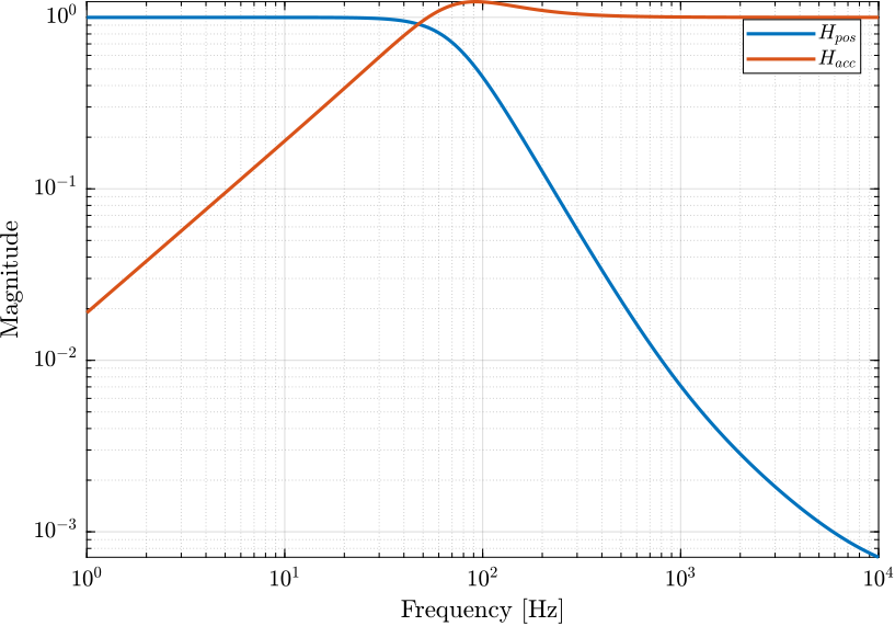
H1 = 1 - H2;The complementary filters obtained are shown on figure fig:htwo_comp_filters.
Sensor Noise
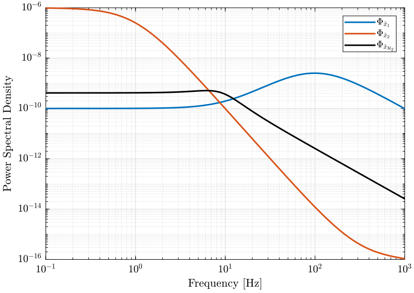
The PSD of the noise of the individual sensor and of the super sensor are shown in Fig. fig:psd_sensors_htwo_synthesis.
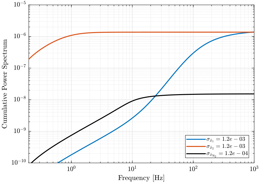
The Cumulative Power Spectrum (CPS) is shown on Fig. fig:cps_h2_synthesis.
The obtained RMS value of the super sensor is lower than the RMS value of the individual sensors.
  PSD_S1 = abs(squeeze(freqresp(N1, freqs, 'Hz'))).^2;
  PSD_S2 = abs(squeeze(freqresp(N2, freqs, 'Hz'))).^2;
  PSD_H2 = abs(squeeze(freqresp(N1*H1, freqs, 'Hz'))).^2+abs(squeeze(freqresp(N2*H2, freqs, 'Hz'))).^2;

  CPS_S1 = cumtrapz(freqs, PSD_S1);
  CPS_S2 = cumtrapz(freqs, PSD_S2);
CPS_H2 = cumtrapz(freqs, PSD_H2);| RMS [m/s] | |
|---|---|
| Integrated Acceleration | 0.005 |
| Derived Position | 0.08 |
| Super Sensor - $\mathcal{H}_2$ | 0.0012 |
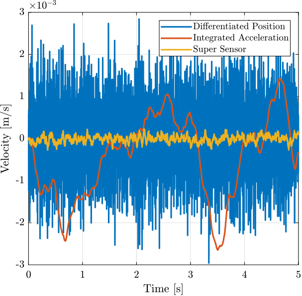
Time Domain Simulation
Parameters of the time domain simulation.
  Fs = 1e4; % Sampling Frequency [Hz]
  Ts = 1/Fs; % Sampling Time [s]

  t = 0:Ts:2; % Time Vector [s]
Time domain velocity.
v = 0.1*sin((10*t).*t)';Generate noises in velocity corresponding to sensor 1 and 2:
  n1 = lsim(N1, sqrt(Fs/2)*randn(length(t), 1), t);
n2 = lsim(N2, sqrt(Fs/2)*randn(length(t), 1), t);Discrepancy between sensor dynamics and model
Conclusion
From the above complementary filter design with the $\mathcal{H}_2$ and $\mathcal{H}_\infty$ synthesis, it still seems that the $\mathcal{H}_2$ synthesis gives the complementary filters that permits to obtain the minimal super sensor noise (when measuring with the $\mathcal{H}_2$ norm).
However, the synthesis does not take into account the robustness of the sensor fusion.
Robust Sensor Fusion: $\mathcal{H}_\infty$ Synthesis with Acc and Pos
<<sec:comp_filter_robustness>>
Introduction ignore
We initially considered perfectly known sensor dynamics so that it can be perfectly inverted.
We now take into account the fact that the sensor dynamics is only partially known. To do so, we model the uncertainty that we have on the sensor dynamics by multiplicative input uncertainty as shown in Fig. fig:sensor_fusion_dynamic_uncertainty.

The objective here is to design complementary filters $H_1(s)$ and $H_2(s)$ in order to minimize the dynamical uncertainty of the super sensor.
ZIP file containing the data and matlab files ignore
The Matlab scripts is accessible here.
Super Sensor Dynamical Uncertainty
In practical systems, the sensor dynamics has always some level of uncertainty. Let's represent that with multiplicative input uncertainty as shown on figure fig:sensor_fusion_dynamic_uncertainty.

The dynamics of the super sensor is represented by
\begin{align*} \frac{\hat{x}}{x} &= (1 + W_1 \Delta_1) H_1 + (1 + W_2 \Delta_2) H_2 \\ &= 1 + W_1 H_1 \Delta_1 + W_2 H_2 \Delta_2 \end{align*}with $\Delta_i$ is any transfer function satisfying $\| \Delta_i \|_\infty < 1$.
We see that as soon as we have some uncertainty in the sensor dynamics, we have that the complementary filters have some effect on the transfer function from $x$ to $\hat{x}$.
The uncertainty set of the transfer function from $\hat{x}$ to $x$ at frequency $\omega$ is bounded in the complex plane by a circle centered on 1 and with a radius equal to $|W_1(j\omega) H_1(j\omega)| + |W_2(j\omega) H_2(j\omega)|$ (figure fig:uncertainty_gain_phase_variation).
We then have that the angle introduced by the super sensor is bounded by $\arcsin(\epsilon)$: \[ \angle \frac{\hat{x}}{x}(j\omega) \le \arcsin \Big(|W_1(j\omega) H_1(j\omega)| + |W_2(j\omega) H_2(j\omega)|\Big) \]

Synthesis objective
The uncertainty region of the super sensor dynamics is represented by a circle in the complex plane as shown in Fig. fig:uncertainty_gain_phase_variation.
At each frequency $\omega$, the radius of the circle is $|W_1(j\omega) H_1(j\omega)| + |W_2(j\omega) H_2(j\omega)|$.
Thus, the phase shift $\Delta\phi(\omega)$ due to the super sensor uncertainty is bounded by: \[ |\Delta\phi(\omega)| \leq \arcsin\big( |W_1(j\omega) H_1(j\omega)| + |W_2(j\omega) H_2(j\omega)| \big) \]
Let's define some allowed frequency depend phase shift $\Delta\phi_\text{max}(\omega) > 0$ such that: \[ |\Delta\phi(\omega)| < \Delta\phi_\text{max}(\omega), \quad \forall\omega \]
If $H_1(s)$ and $H_2(s)$ are designed such that \[ |W_1(j\omega) H_1(j\omega)| + |W_2(j\omega) H_2(j\omega)| < \sin\big( \Delta\phi_\text{max}(\omega) \big) \]
The maximum phase shift due to dynamic uncertainty at frequency $\omega$ will be $\Delta\phi_\text{max}(\omega)$.
Requirements as an $\mathcal{H}_\infty$ norm
We now try to express this requirement in terms of an $\mathcal{H}_\infty$ norm.
Let's define one weight $W_\phi(s)$ that represents the maximum wanted phase uncertainty: \[ |W_{\phi}(j\omega)|^{-1} \approx \sin(\Delta\phi_{\text{max}}(\omega)), \quad \forall\omega \]
Then:
\begin{align*} & |W_1(j\omega) H_1(j\omega)| + |W_2(j\omega) H_2(j\omega)| < \sin\big( \Delta\phi_\text{max}(\omega) \big), \quad \forall\omega \\ \Longleftrightarrow & |W_1(j\omega) H_1(j\omega)| + |W_2(j\omega) H_2(j\omega)| < |W_\phi(j\omega)|^{-1}, \quad \forall\omega \\ \Longleftrightarrow & \left| W_1(j\omega) H_1(j\omega) W_\phi(j\omega) \right| + \left| W_2(j\omega) H_2(j\omega) W_\phi(j\omega) \right| < 1, \quad \forall\omega \end{align*}Which is approximately equivalent to (with an error of maximum $\sqrt{2}$):
\begin{equation} \left\| \begin{matrix} W_1(s) W_\phi(s) H_1(s) \\ W_2(s) W_\phi(s) H_2(s) \end{matrix} \right\|_\infty < 1 \end{equation}One should not forget that at frequency where both sensors has unknown dynamics ($|W_1(j\omega)| > 1$ and $|W_2(j\omega)| > 1$), the super sensor dynamics will also be unknown and the phase uncertainty cannot be bounded. Thus, at these frequencies, $|W_\phi|$ should be smaller than $1$.
Weighting Function used to bound the super sensor uncertainty
Let's define $W_\phi(s)$ in order to bound the maximum allowed phase uncertainty $\Delta\phi_\text{max}$ of the super sensor dynamics. The magnitude $|W_\phi(j\omega)|$ is shown in Fig. fig:magnitude_wphi and the corresponding maximum allowed phase uncertainty of the super sensor dynamics of shown in Fig. fig:maximum_wanted_phase_uncertainty.
  Dphi = 10; % [deg]

Wu = createWeight('n', 2, 'w0', 2*pi*4e2, 'G0', 1/sin(Dphi*pi/180), 'G1', 1/4, 'Gc', 1); save('./mat/Wu.mat', 'Wu');The obtained upper bounds on the complementary filters in order to limit the phase uncertainty of the super sensor are represented in Fig. fig:upper_bounds_comp_filter_max_phase_uncertainty.
<<plt-matlab>>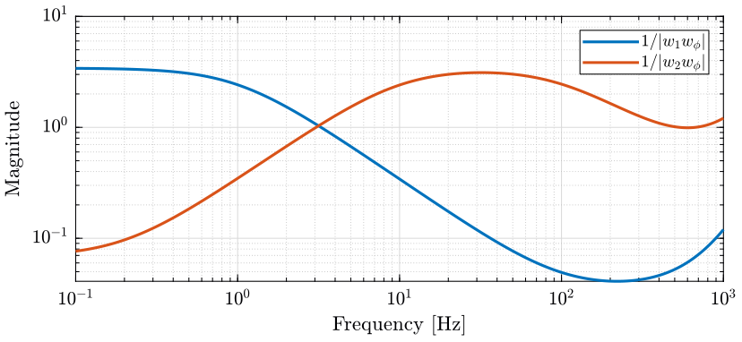
$\mathcal{H}_\infty$ Synthesis
The $\mathcal{H}_\infty$ synthesis architecture used for the complementary filters is shown in Fig. fig:h_infinity_robust_fusion.

The generalized plant is defined below.
  P = [Wu*W1 -Wu*W1;
       0       Wu*W2;
       1       0];
And we do the $\mathcal{H}_\infty$ synthesis using the hinfsyn command.
[H2, ~, gamma, ~] = hinfsyn(P, 1, 1,'TOLGAM', 0.001, 'METHOD', 'ric', 'DISPLAY', 'on');[H2, ~, gamma, ~] = hinfsyn(P, 1, 1,'TOLGAM', 0.001, 'METHOD', 'ric', 'DISPLAY', 'on');
Test bounds: 0.7071 <= gamma <= 1.291
gamma X>=0 Y>=0 rho(XY)<1 p/f
9.554e-01 0.0e+00 0.0e+00 3.529e-16 p
8.219e-01 0.0e+00 0.0e+00 5.204e-16 p
7.624e-01 3.8e-17 0.0e+00 1.955e-15 p
7.342e-01 0.0e+00 0.0e+00 5.612e-16 p
7.205e-01 0.0e+00 0.0e+00 7.184e-16 p
7.138e-01 0.0e+00 0.0e+00 0.000e+00 p
7.104e-01 4.1e-16 0.0e+00 6.749e-15 p
7.088e-01 0.0e+00 0.0e+00 2.794e-15 p
7.079e-01 0.0e+00 0.0e+00 6.503e-16 p
7.075e-01 0.0e+00 0.0e+00 4.302e-15 p
Best performance (actual): 0.7071
And $H_1(s)$ is defined as the complementary of $H_2(s)$.
H1 = 1 - H2;The obtained complementary filters are shown in Fig. fig:comp_filter_hinf_uncertainty.
<<plt-matlab>>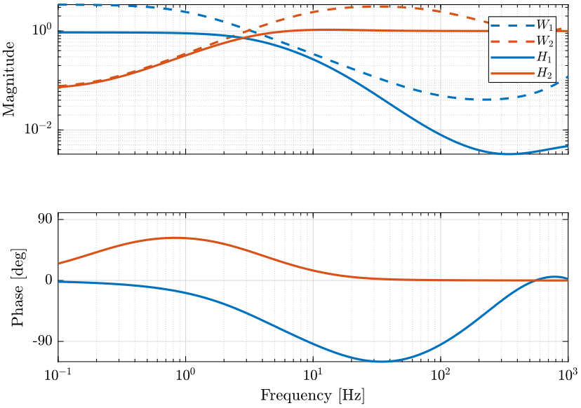
Super sensor uncertainty
We can now compute the uncertainty of the super sensor. The result is shown in Fig. fig:super_sensor_uncertainty_bode_plot.
H2_filters = load('./mat/H2_filters.mat', 'H2', 'H1');The uncertainty of the super sensor cannot be made smaller than both the individual sensor. Ideally, it would follow the minimum uncertainty of both sensors.
We here just used very wimple weights. For instance, we could improve the dynamical uncertainty of the super sensor by making $|W_\phi(j\omega)|$ smaller bellow 2Hz where the dynamical uncertainty of the sensor 1 is small.
Super sensor noise
We now compute the obtain Power Spectral Density of the super sensor's noise. The noise characteristics of both individual sensor are defined below.
The PSD of both sensor and of the super sensor is shown in Fig. fig:psd_sensors_hinf_synthesis. The CPS of both sensor and of the super sensor is shown in Fig. fig:cps_sensors_hinf_synthesis.
  PSD_S2   = abs(squeeze(freqresp(N2, freqs, 'Hz'))).^2;
  PSD_S1   = abs(squeeze(freqresp(N1, freqs, 'Hz'))).^2;
  PSD_Hinf = abs(squeeze(freqresp(N1*H1, freqs, 'Hz'))).^2+abs(squeeze(freqresp(N2*H2, freqs, 'Hz'))).^2;
  PSD_H2   = abs(squeeze(freqresp(N1*H2_filters.H1, freqs, 'Hz'))).^2+abs(squeeze(freqresp(N2*H2_filters.H2, freqs, 'Hz'))).^2;

  CPS_S2   = cumtrapz(freqs, PSD_S2);
  CPS_S1   = cumtrapz(freqs, PSD_S1);
  CPS_Hinf = cumtrapz(freqs, PSD_Hinf);
CPS_H2 = cumtrapz(freqs, PSD_H2); <<plt-matlab>>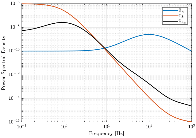
<<plt-matlab>>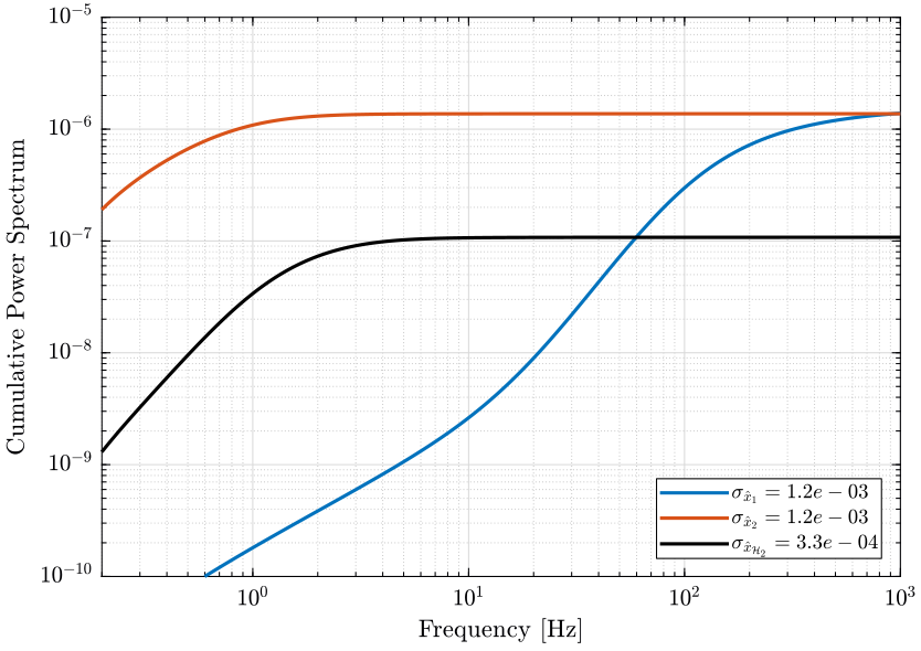
Conclusion
Using the $\mathcal{H}_\infty$ synthesis, the dynamical uncertainty of the super sensor can be bounded to acceptable values.
However, the RMS of the super sensor noise is not optimized as it was the case with the $\mathcal{H}_2$ synthesis
Optimal and Robust Sensor Fusion: Mixed $\mathcal{H}_2/\mathcal{H}_\infty$ Synthesis with Acc and Pos
<<sec:mixed_synthesis_sensor_fusion>>
ZIP file containing the data and matlab files ignore
The Matlab scripts is accessible here.
Mixed $\mathcal{H}_2$ / $\mathcal{H}_\infty$ Synthesis - Introduction
The goal is to design complementary filters such that:
- the maximum uncertainty of the super sensor is bounded
- the RMS value of the super sensor noise is minimized
To do so, we can use the Mixed $\mathcal{H}_2$ / $\mathcal{H}_\infty$ Synthesis.
The Matlab function for that is h2hinfsyn (doc).
Noise characteristics and Uncertainty of the individual sensors
Both dynamical uncertainty and noise characteristics of the individual sensors are shown in Fig. fig:mixed_synthesis_noise_uncertainty_sensors.
<<plt-matlab>>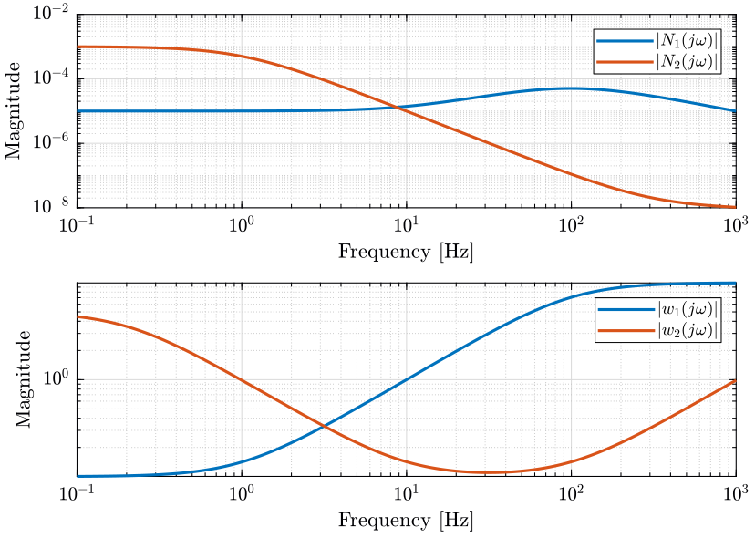
Weighting Functions on the uncertainty of the super sensor
We design weights for the $\mathcal{H}_\infty$ part of the synthesis in order to limit the dynamical uncertainty of the super sensor. The maximum wanted multiplicative uncertainty is shown in Fig. fig:mixed_syn_hinf_weight. The idea here is that we don't really need low uncertainty at low frequency but only near the crossover frequency that is suppose to be around 300Hz here.
Mixed $\mathcal{H}_2$ / $\mathcal{H}_\infty$ Synthesis
The synthesis architecture that is used here is shown in Fig. fig:mixed_h2_hinf_synthesis.
The controller $K$ is synthesized such that it:
- Keeps the $\mathcal{H}_\infty$ norm $G$ of the transfer function from $w$ to $z_\infty$ bellow some specified value
- Keeps the $\mathcal{H}_2$ norm $H$ of the transfer function from $w$ to $z_2$ bellow some specified value
- Minimizes a trade-off criterion of the form $W_1 G^2 + W_2 H^2$ where $W_1$ and $W_2$ are specified values

Here, we define $P$ such that:
\begin{align*} \left\| \frac{z_\infty}{w} \right\|_\infty &= \left\| \begin{matrix}W_1(s) H_1(s) \\ W_2(s) H_2(s)\end{matrix} \right\|_\infty \\ \left\| \frac{z_2}{w} \right\|_2 &= \left\| \begin{matrix}N_1(s) H_1(s) \\ N_2(s) H_2(s)\end{matrix} \right\|_2 \end{align*}Then:
- we specify the maximum value for the $\mathcal{H}_\infty$ norm between $w$ and $z_\infty$ to be $1$
- we don't specify any maximum value for the $\mathcal{H}_2$ norm between $w$ and $z_2$
- we choose $W_1 = 0$ and $W_2 = 1$ such that the objective is to minimize the $\mathcal{H}_2$ norm between $w$ and $z_2$
The synthesis objective is to have: \[ \left\| \frac{z_\infty}{w} \right\|_\infty = \left\| \begin{matrix}W_1(s) H_1(s) \\ W_2(s) H_2(s)\end{matrix} \right\|_\infty < 1 \] and to minimize: \[ \left\| \frac{z_2}{w} \right\|_2 = \left\| \begin{matrix}N_1(s) H_1(s) \\ N_2(s) H_2(s)\end{matrix} \right\|_2 \] which is what we wanted.
We define the generalized plant that will be used for the mixed synthesis.
  W1u = ss(W2*Wu); W2u = ss(W1*Wu); % Weight on the uncertainty
  W1n = ss(N2); W2n = ss(N1); % Weight on the noise

  P = [W1u -W1u;
       0    W2u;
       W1n -W1n;
       0    W2n;
       1    0];
The mixed $\mathcal{H}_2/\mathcal{H}_\infty$ synthesis is performed below.
  Nmeas = 1; Ncon = 1; Nz2 = 2;

  [H1, ~, normz, ~] = h2hinfsyn(P, Nmeas, Ncon, Nz2, [0, 1], 'HINFMAX', 1, 'H2MAX', Inf, 'DKMAX', 100, 'TOL', 0.01, 'DISPLAY', 'on');

  H2 = 1 - H1;
The obtained complementary filters are shown in Fig. fig:comp_filters_mixed_synthesis.
<<plt-matlab>>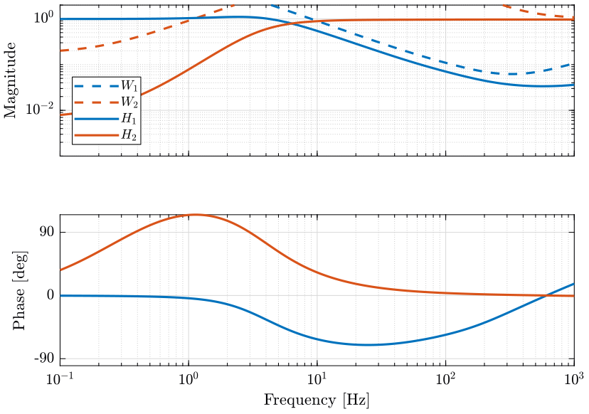
Obtained Super Sensor's noise
The PSD and CPS of the super sensor's noise are shown in Fig. fig:psd_super_sensor_mixed_syn and Fig. fig:cps_super_sensor_mixed_syn respectively.
  PSD_S2     = abs(squeeze(freqresp(N2, freqs, 'Hz'))).^2;
  PSD_S1     = abs(squeeze(freqresp(N1, freqs, 'Hz'))).^2;
  PSD_H2Hinf = abs(squeeze(freqresp(N1*H1, freqs, 'Hz'))).^2+abs(squeeze(freqresp(N2*H2, freqs, 'Hz'))).^2;

  CPS_S2     = cumtrapz(freqs, PSD_S2);
  CPS_S1     = cumtrapz(freqs, PSD_S1);
CPS_H2Hinf = cumtrapz(freqs, PSD_H2Hinf); <<plt-matlab>>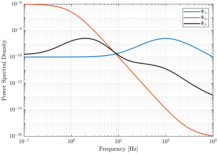
<<plt-matlab>>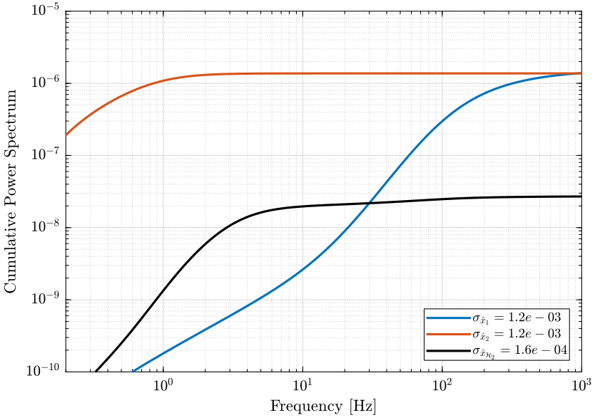
Obtained Super Sensor's Uncertainty
The uncertainty on the super sensor's dynamics is shown in Fig. fig:super_sensor_dyn_uncertainty_mixed_syn.
Comparison Hinf H2 H2/Hinf
  H2_filters      = load('./mat/H2_filters.mat',      'H2', 'H1');
  Hinf_filters    = load('./mat/Hinf_filters.mat',    'H2', 'H1');
  H2_Hinf_filters = load('./mat/H2_Hinf_filters.mat', 'H2', 'H1');
PSD_H2 = abs(squeeze(freqresp(N2*H2_filters.H2, freqs, 'Hz'))).^2+abs(squeeze(freqresp(N1*H2_filters.H1, freqs, 'Hz'))).^2;
CPS_H2 = cumtrapz(freqs, PSD_H2);
PSD_Hinf = abs(squeeze(freqresp(N2*Hinf_filters.H2, freqs, 'Hz'))).^2+abs(squeeze(freqresp(N1*Hinf_filters.H1, freqs, 'Hz'))).^2;
CPS_Hinf = cumtrapz(freqs, PSD_Hinf);
PSD_H2Hinf = abs(squeeze(freqresp(N2*H2_Hinf_filters.H2, freqs, 'Hz'))).^2+abs(squeeze(freqresp(N1*H2_Hinf_filters.H1, freqs, 'Hz'))).^2;
CPS_H2Hinf = cumtrapz(freqs, PSD_H2Hinf);| RMS [m/s] | |
|---|---|
| Optimal: $\mathcal{H}_2$ | 0.0012 |
| Robust: $\mathcal{H}_\infty$ | 0.041 |
| Mixed: $\mathcal{H}_2/\mathcal{H}_\infty$ | 0.011 |
Conclusion
This synthesis methods allows both to:
- limit the dynamical uncertainty of the super sensor
- minimize the RMS value of the estimation
Functions
createWeight
<<sec:createWeight>>
This Matlab function is accessible here.
    function [W] = createWeight(args)
    % createWeight -
    %
    % Syntax: [in_data] = createWeight(in_data)
    %
    % Inputs:
    %    - n  - Weight Order
    %    - G0 - Low frequency Gain
    %    - G1 - High frequency Gain
    %    - Gc - Gain of W at frequency w0
    %    - w0 - Frequency at which |W(j w0)| = Gc
    %
    % Outputs:
    %    - W - Generated Weight

        arguments
            args.n  (1,1) double {mustBeInteger, mustBePositive} = 1
            args.G0 (1,1) double {mustBeNumeric, mustBePositive} = 0.1
            args.G1 (1,1) double {mustBeNumeric, mustBePositive} = 10
            args.Gc (1,1) double {mustBeNumeric, mustBePositive} = 1
            args.w0 (1,1) double {mustBeNumeric, mustBePositive} = 1
        end

      mustBeBetween(args.G0, args.Gc, args.G1);

      s = tf('s');

      W = (((1/args.w0)*sqrt((1-(args.G0/args.Gc)^(2/args.n))/(1-(args.Gc/args.G1)^(2/args.n)))*s + (args.G0/args.Gc)^(1/args.n))/((1/args.G1)^(1/args.n)*(1/args.w0)*sqrt((1-(args.G0/args.Gc)^(2/args.n))/(1-(args.Gc/args.G1)^(2/args.n)))*s + (1/args.Gc)^(1/args.n)))^args.n;

      end

      % Custom validation function
      function mustBeBetween(a,b,c)
          if ~((a > b && b > c) || (c > b && b > a))
              eid = 'createWeight:inputError';
              msg = 'Gc should be between G0 and G1.';
              throwAsCaller(MException(eid,msg))
          end
      end
plotMagUncertainty
<<sec:plotMagUncertainty>>
This Matlab function is accessible here.
  function [p] = plotMagUncertainty(W, freqs, args)
  % plotMagUncertainty -
  %
  % Syntax: [p] = plotMagUncertainty(W, freqs, args)
  %
  % Inputs:
  %    - W     - Multiplicative Uncertainty Weight
  %    - freqs - Frequency Vector [Hz]
  %    - args  - Optional Arguments:
  %      - G
  %      - color_i
  %      - opacity
  %
  % Outputs:
  %    - p - Plot Handle

  arguments
      W
      freqs double {mustBeNumeric, mustBeNonnegative}
      args.G = tf(1)
      args.color_i (1,1) double {mustBeInteger, mustBePositive} = 1
      args.opacity (1,1) double {mustBeNumeric, mustBePositive} = 0.3
      args.DisplayName char = ''
  end

  % Get defaults colors
  colors = get(groot, 'defaultAxesColorOrder');

  p = patch([freqs flip(freqs)], ...
            [abs(squeeze(freqresp(args.G, freqs, 'Hz'))).*(1 + abs(squeeze(freqresp(W, freqs, 'Hz')))); ...
             flip(abs(squeeze(freqresp(args.G, freqs, 'Hz'))).*max(1 - abs(squeeze(freqresp(W, freqs, 'Hz'))), 1e-6))], 'w', ...
            'DisplayName', args.DisplayName);

  p.FaceColor = colors(args.color_i, :);
  p.EdgeColor = 'none';
  p.FaceAlpha = args.opacity;

  end
plotPhaseUncertainty
<<sec:plotPhaseUncertainty>>
This Matlab function is accessible here.
  function [p] = plotPhaseUncertainty(W, freqs, args)
  % plotPhaseUncertainty -
  %
  % Syntax: [p] = plotPhaseUncertainty(W, freqs, args)
  %
  % Inputs:
  %    - W     - Multiplicative Uncertainty Weight
  %    - freqs - Frequency Vector [Hz]
  %    - args  - Optional Arguments:
  %      - G
  %      - color_i
  %      - opacity
  %
  % Outputs:
  %    - p - Plot Handle

  arguments
      W
      freqs double {mustBeNumeric, mustBeNonnegative}
      args.G = tf(1)
      args.color_i (1,1) double {mustBeInteger, mustBePositive} = 1
      args.opacity (1,1) double {mustBeNumeric, mustBePositive} = 0.3
      args.DisplayName char = ''
  end

  % Get defaults colors
  colors = get(groot, 'defaultAxesColorOrder');

  % Compute Phase Uncertainty
  Dphi = 180/pi*asin(abs(squeeze(freqresp(W, freqs, 'Hz'))));
  Dphi(abs(squeeze(freqresp(W, freqs, 'Hz'))) > 1) = 360;

  % Compute Plant Phase
  G_ang = 180/pi*angle(squeeze(freqresp(args.G, freqs, 'Hz')));

  p = patch([freqs flip(freqs)], [G_ang+Dphi; flip(G_ang-Dphi)], 'w', ...
            'DisplayName', args.DisplayName);

  p.FaceColor = colors(args.color_i, :);
  p.EdgeColor = 'none';
  p.FaceAlpha = args.opacity;

  end
Bibliography ignore
bibliographystyle:unsrt bibliography:ref.bib
