dcm-stepper-calibration/dcm_lookup_tables.org

ESRF Double Crystal Monochromator - Lookup Tables

• Introduction
• Stepper Motors Calibration
  • Introduction
  • Schematic
  • Patterns in the Fast Jack motion errors
  • Experimental Data - Current Method
  • Simulation
  • Experimental Data - Proposed method
• Attocube Calibration
  • Introduction
  • Simulations
• Bibliography

---

This report is also available as a pdf.

---

Introduction   ignore

Several Lookup Tables (LUT) are used for the DCM in order to compensate for repeatable errors.

• Section sec:dcm_stepper_lut: the stepper motors are calibrated using interferometers.
• Section sec:dcm_attocube_lut: the Attocube periodic non-linearities are calibrated using piezoelectric actuators.

Stepper Motors Calibration

<<sec:dcm_stepper_lut>>

Introduction   ignore

Fast jack coarse displacement is performed with a Stepper motor and a ball screw mechanism. Such positioning system has some repeatable motion errors than can be calibrated using a measurement system having less errors.

For the DCM, this can be done using the interferometers.

Schematic

In order to measure the errors induced by the fast jacks, we have to make some scans, and measure simultaneously:

• The wanted fast jack position: signal/step sent by the IcePAP
• The actual (measured) position

The experimental setup to perform this is shown in Figure fig:block_diagram_lut_stepper.

The procedure is the following:

• A scan on the Bragg angle $\theta$ is generated from Bliss
• Reference paths $[r_{u_r},\ r_{u_h},\ r_{d}]$ are sent to the IcePAP
• Initially, the LUT inside the IcePAP is not changing the reference path
• The IcePAP generates some steps $[u_{u_r},\ u_{u_h},\ u_{d}]$ that are sent to the fast jacks
• The motion of the crystals $[d_z,\ r_y,\ r_x]$ is measured with the interferometers and computed in the Speedgoat
• Finally, the corresponding motion $[d_{u_r},\ r_{u_h},\ r_d]$ of the fast jack is computed afterwards in BLISS

The measured motion of the fast jacks $[d_{u_r},\ r_{u_h},\ r_d]$ can be compared with the IcePAP steps $[u_{u_r},\ u_{u_h},\ u_{d}]$ in order to create the LUT inside the IcePAP.

\definecolor{myblue}{rgb}{0, 0.447, 0.741}
\definecolor{myred}{rgb}{0.8500, 0.325, 0.098}
\definecolor{mygreen}{rgb}{0.639, 0.745, 0.549}
\definecolor{myyellow}{rgb}{0.922, 0.796, 0.545}

\begin{tikzpicture}
  % Blocks
  \node[block={1.5cm}{2.9cm}] (traj) at (0,0){$\frac{d_{\text{off}}}{2 \cos \theta}$};

  \node[block={1.5cm}{0.8cm}, right=1.1   of traj] (lut_uh) {LUT $u_h$};
  \node[block={1.5cm}{0.8cm}, above=0.2 of lut_uh] (lut_ur) {LUT $u_r$};
  \node[block={1.5cm}{0.8cm}, below=0.2 of lut_uh] (lut_d)  {LUT $d$};

  \node[block={1.5cm}{0.8cm}, right=1.1 of lut_ur] (fj_ur) {FJ $u_h$};
  \node[block={1.5cm}{0.8cm}, right=1.1 of lut_uh] (fj_uh) {FJ $u_r$};
  \node[block={1.5cm}{0.8cm}, right=1.1 of lut_d]  (fj_d)  {FJ $d$};

  \node[block={1.5cm}{2.9cm}, right=0.2 of fj_uh] (int) {\rotatebox{90}{Interferometers}};

  \node[block={1.5cm}{2.9cm}, right=0.6 of int] (Js) {\rotatebox{90}{\parbox[c]{2.0cm}{\centering Forward Kinematics}}};

  \node[block={1.5cm}{2.9cm}, right=1.1 of Js] (Ja) {\rotatebox{90}{\parbox[c]{2.0cm}{\centering Inverse Kinematics}}};

  % Signals
  \draw[->] ($(traj.west) + (-0.7, 0)$)node[above right]{$\theta$} -- (traj.west);

  \draw[->] (lut_ur-|traj.east) --node[midway, above]{$r_{u_r}$} (lut_ur.west);
  \draw[->] (lut_uh-|traj.east) --node[midway, above]{$r_{u_h}$} (lut_uh.west);
  \draw[->] (lut_d -|traj.east) --node[midway, above]{$r_{d}$}   (lut_d.west);

  \draw[->] (lut_ur.east) --node[midway, above]{$u_{u_r}$} (fj_ur.west);
  \draw[->] (lut_uh.east) --node[midway, above]{$u_{u_h}$} (fj_uh.west);
  \draw[->] (lut_d.east)  --node[midway, above]{$u_{d}$}   (fj_d.west);

  \draw[->] (int.east) -- (Js.west);

  \draw[->] (Js.east|-fj_ur) --node[midway, above]{$d_z$} (Ja.west|-fj_ur);
  \draw[->] (Js.east|-fj_uh) --node[midway, above]{$r_y$} (Ja.west|-fj_uh);
  \draw[->] (Js.east|-fj_d)  --node[midway, above]{$r_x$} (Ja.west|-fj_d) ;

  \draw[->] (Ja.east|-fj_ur) -- ++(1.0, 0)node[above left]{$d_{u_r}$};
  \draw[->] (Ja.east|-fj_uh) -- ++(1.0, 0)node[above left]{$d_{u_h}$};
  \draw[->] (Ja.east|-fj_d)  -- ++(1.0, 0)node[above left]{$d_{d}$};

  \begin{scope}[on background layer]
    \node[fit={(fj_d.south west) (int.north east)}, fill=myblue!20!white, draw, inner sep=6pt] (dcm) {};
    \node[fit={(Js.south west) (Js.north east)}, fill=myyellow!20!white, draw, inner sep=6pt] (speedgoat) {};
    \node[fit={(lut_d.south west) (lut_ur.north east)}, fill=myred!20!white, draw, inner sep=6pt] (icepap) {};
    \node[fit={(traj.south west) (traj.north east)}, fill=mygreen!20!white, draw, inner sep=6pt] (bliss_1) {};
    \node[fit={(Ja.south west) (Ja.north east)}, fill=mygreen!20!white, draw, inner sep=6pt] (bliss_2) {};
    \node[above] at (dcm.north) {DCM};
    \node[above] at (speedgoat.north) {Speedgoat};
    \node[above] at (icepap.north) {IcePAP};
    \node[above] at (bliss_1.north) {BLISS};
    \node[above] at (bliss_2.north) {BLISS};
  \end{scope}
\end{tikzpicture}

Block diagram of the experiment to create the Lookup Table

Patterns in the Fast Jack motion errors

In order to understand what should be the "sampling distance" for the lookup table of the stepper motor, we have to analyze the displacement errors induced by the stepper motor.

Let's load the measurements of one bragg angle scan without any LUT.

%% Load Data of the new LUT method
ol_bragg = (pi/180)*1e-5*double(h5read('Qutools_test_0001.h5','/33.1/instrument/trajmot/data')); % Bragg angle [rad]
ol_dzw   = 10.5e-3./(2*cos(ol_bragg)); % Wanted distance between crystals [m]

ol_dz    = 1e-9*double(h5read('Qutools_test_0001.h5','/33.1/instrument/xtal_111_dz_filter/data'));  % Dz distance between crystals [m]
ol_dry   = 1e-9*double(h5read('Qutools_test_0001.h5','/33.1/instrument/xtal_111_dry_filter/data')); % Ry [rad]
ol_drx   = 1e-9*double(h5read('Qutools_test_0001.h5','/33.1/instrument/xtal_111_drx_filter/data')); % Rx [rad]

ol_t = 1e-6*double(h5read('Qutools_test_0001.h5','/33.1/instrument/time/data')); % Time [s]

ol_ddz   = ol_fj-ol_dz; % Distance Error between crystals [m]

Orientation and Distance error of the Crystal measured by the interferometers

Now let's convert the errors from the frame of the crystal to the frame of the fast jacks (inverse kinematics problem) using the Jacobian matrix.

%% Compute Fast Jack position errors
% Jacobian matrix for Fast Jacks and 111 crystal
J_a_111 = [1,  0.14, -0.1525
           1,  0.14,  0.0675
           1, -0.14,  0.0425];

ol_de_111 = [ol_ddz'; ol_dry'; ol_drx'];

% Fast Jack position errors
ol_de_fj = J_a_111*ol_de_111;

ol_fj_ur = ol_de_fj(1,:);
ol_fj_uh = ol_de_fj(2,:);
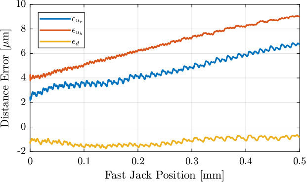
ol_fj_d  = ol_de_fj(3,:);

Estimated motion errors of the fast jacks during the scan

Let's now identify this pattern as a function of the fast-jack position.

As we want to done frequency Fourier transform, we need to have uniform sampling along the fast jack position. To do so, the function resample is used.

Xs = 0.1e-6; % Sampling Distance [m]

%% Re-sampled data with uniform spacing [m]
ol_fj_ur_u = resample(ol_fj_ur, ol_dzw, 1/Xs);
ol_fj_uh_u = resample(ol_fj_uh, ol_dzw, 1/Xs);
ol_fj_d_u  = resample(ol_fj_d,  ol_dzw, 1/Xs);

ol_fj_u = Xs*[1:length(ol_fj_ur_u)]; % Sampled Jack Position

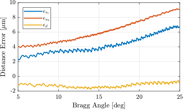
The result is shown in Figure fig:exp_without_lut_fj_pos_errors_distance.

Position error of fast jacks as a function of the fast jack motion

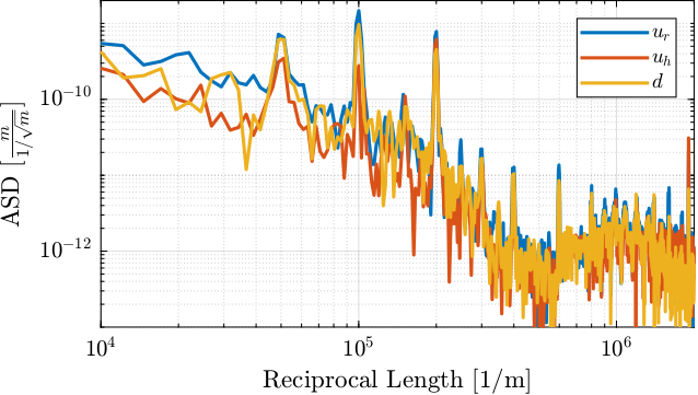
Let's now perform a Power Spectral Analysis of the measured displacement errors of the Fast Jack.

% Hanning Windows with 250um width
win = hanning(floor(400e-6/Xs));

% Power Spectral Density [m2/(1/m)]
[S_fj_ur, f] = pwelch(ol_fj_ur_u-mean(ol_fj_ur_u), win, 0, [], 1/Xs);
[S_fj_uh, ~] = pwelch(ol_fj_uh_u-mean(ol_fj_uh_u), win, 0, [], 1/Xs);
[S_fj_d,  ~] = pwelch(ol_fj_d_u -mean(ol_fj_d_u ),  win, 0, [], 1/Xs);

As shown in Figure fig:exp_without_lut_wavenumber_asd, we can see a fundamental "reciprocal length" of $5 \cdot 10^4\,[1/m]$ and its harmonics. This corresponds to a length of $\frac{1}{5\cdot 10^4} = 20\,[\mu m]$.

Spectral content of the error as a function of the reciprocal length

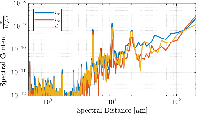
Instead of looking at that as a function of the reciprocal length, we can look at it as a function of the spectral distance (Figure fig:exp_without_lut_spectral_content_fj_error).

We see that the errors have a pattern with "spectral distances" equal to $5\,[\mu m]$, $10\,[\mu m]$, $20\,[\mu m]$ and smaller harmonics.

Spectral content of the error as a function of the spectral distance

Let's try to understand these results. One turn of the stepper motor corresponds to a vertical motion of 1mm. The stepper motor has 50 pairs of poles, therefore one pair of pole corresponds to a motion of $20\,[\mu m]$ which is the fundamental "spectral distance" we observe.

CPS_ur = flip(-cumtrapz(flip(f), flip(S_fj_ur)));
CPS_uh = flip(-cumtrapz(flip(f), flip(S_fj_uh)));
CPS_d  = flip(-cumtrapz(flip(f), flip(S_fj_d)));

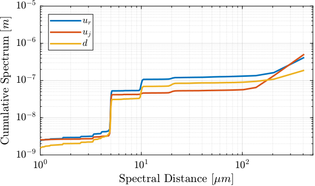
From Figure fig:exp_without_lut_cas_pos_error, we can see that if the motion errors with a period of $5\,[\mu m]$ and $10\,[\mu m]$ can be dealt with the lookup table, this will reduce a lot the positioning errors of the fast jack.

%% Cumulative Spectrum
figure;
hold on;
plot(1e6./f, sqrt(CPS_ur), 'DisplayName', '$u_r$');
plot(1e6./f, sqrt(CPS_uh), 'DisplayName', '$u_j$');
plot(1e6./f, sqrt(CPS_d),  'DisplayName', '$d$');
hold off;
set(gca, 'xscale', 'log'); set(gca, 'yscale', 'log');
xlabel('Spectral Distance [$\mu m$]'); ylabel('Cumulative Spectrum [$m$]')
xlim([1, 500]); ylim([1e-9, 1e-5]);
legend('location', 'northwest');

Cumulative spectrum from small spectral distances to large spectral distances

Experimental Data - Current Method

The current used method is an iterative one.

%% Load Experimental Data
ol_bragg    = double(h5read('first_beam_0001.h5','/31.1/instrument/trajmot/data'));
ol_drx      = h5read('first_beam_0001.h5','/31.1/instrument/xtal_111_drx_filter/data');

lut_1_bragg = double(h5read('first_beam_0001.h5','/32.1/instrument/trajmot/data'));
lut_1_drx   = h5read('first_beam_0001.h5','/32.1/instrument/xtal_111_drx_filter/data');

lut_2_bragg = double(h5read('first_beam_0001.h5','/33.1/instrument/trajmot/data'));
lut_2_drx   = h5read('first_beam_0001.h5','/33.1/instrument/xtal_111_drx_filter/data');

lut_3_bragg = double(h5read('first_beam_0001.h5','/34.1/instrument/trajmot/data'));
lut_3_drx   = h5read('first_beam_0001.h5','/34.1/instrument/xtal_111_drx_filter/data');

lut_4_bragg = double(h5read('first_beam_0001.h5','/36.1/instrument/trajmot/data'));
lut_4_drx   = h5read('first_beam_0001.h5','/36.1/instrument/xtal_111_drx_filter/data');

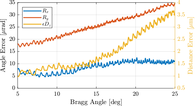
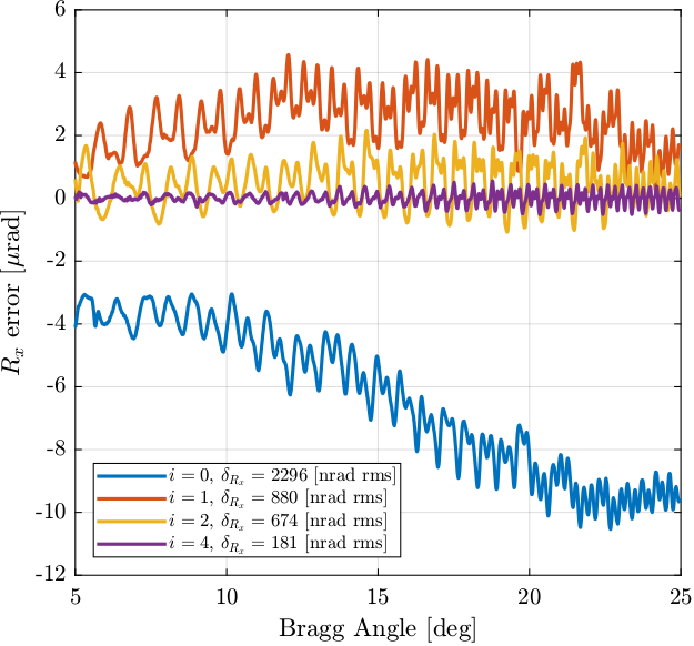
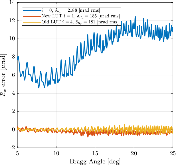
The relative orientation of the two 111 mirrors in the $x$ directions are compared in Figure fig:lut_old_method_exp_data for several iterations. We can see that after the first iteration, the orientation error has an opposite sign as for the case without LUT.

$R_x$ error with the current LUT method

Simulation

In this section, we suppose that we are in the frame of one fast jack (all transformations are already done), and we wish to create a LUT for one fast jack.

Let's say with make a Bragg angle scan between 10deg and 60deg during 100s.

Fs = 10e3; % Sample Frequency [Hz]
t = 0:1/Fs:10; % Time vector [s]
theta = linspace(10, 40, length(t)); % Bragg Angle [deg]

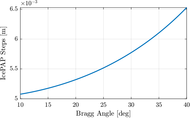
The IcePAP steps are following the theoretical formula:

\begin{equation} d_z = \frac{d_{\text{off}}}{2 \cos \theta} \end{equation}

with $\theta$ the bragg angle and $d_{\text{off}} = 10\,mm$.

The motion to follow is then:

perfect_motion = 10e-3./(2*cos(theta*pi/180)); % Perfect motion [m]

And the IcePAP is generated those steps:

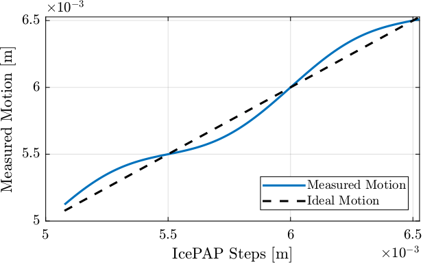
icepap_steps = perfect_motion; % IcePAP steps measured by Speedgoat [m]

IcePAP Steps as a function of the Bragg Angle

Then, we are measuring the motion of the Fast Jack using the Interferometer. The motion error is larger than in reality to be angle to see it more easily.

motion_error = 100e-6*sin(2*pi*perfect_motion/1e-3); % Error motion [m]

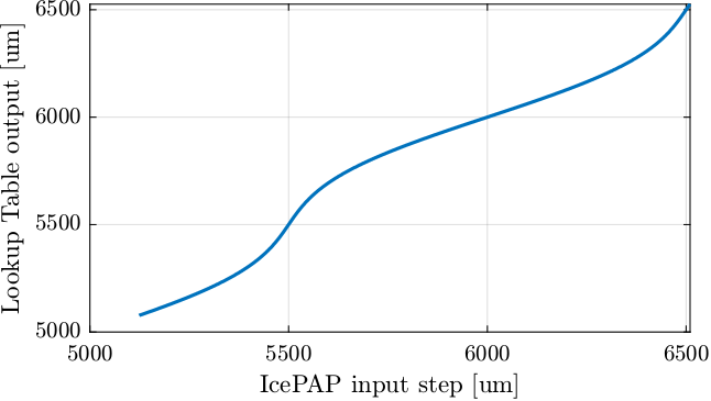
measured_motion = perfect_motion + motion_error; % Measured motion of the Fast Jack [m]

Measured motion as a function of the IcePAP Steps

Let's now compute the lookup table. For each micrometer of the IcePAP step, another step is associated that correspond to a position closer to the wanted position.

%% Get range for the LUT
% We correct only in the range of tested/measured motion
lut_range = round(1e6*min(icepap_steps)):round(1e6*max(icepap_steps)); % IcePAP steps [um]

%% Initialize the LUT
lut = zeros(size(lut_range));

%% For each um in this range
for i = 1:length(lut_range)
    % Get points indices where the measured motion is closed to the wanted one
    close_points = measured_motion > 1e-6*lut_range(i) - 500e-9 & measured_motion < 1e-6*lut_range(i) + 500e-9;
    % Get the corresponding closest IcePAP step
    lut(i) = round(1e6*mean(icepap_steps(close_points))); % [um]
end

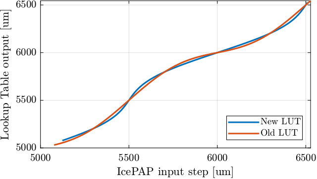
Generated Lookup Table

The current LUT implementation is the following:

motion_error_lut = zeros(size(lut_range));
for i = 1:length(lut_range)
    % Get points indices where the icepap step is close to the wanted one
    close_points = icepap_steps > 1e-6*lut_range(i) - 500e-9 & icepap_steps < 1e-6*lut_range(i) + 500e-9;
    % Get the corresponding motion error
    motion_error_lut(i) = lut_range(i) + (lut_range(i) - round(1e6*mean(measured_motion(close_points)))); % [um]
end

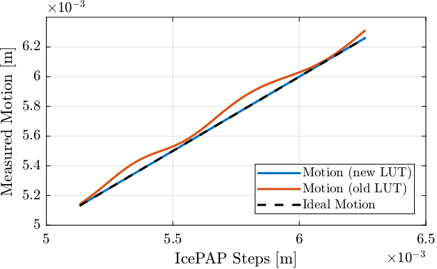
Let's compare the two Lookup Table in Figure fig:lut_comparison_two_methods.

Comparison of the two lookup tables

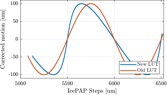
If we plot the "corrected steps" for all steps for both methods, we clearly see the difference (Figure fig:lut_correct_and_motion_error).

LUT correction and motion error as a function of the IcePAP steps

Let's now implement both LUT to see which implementation is correct.

motion_new = zeros(size(icepap_steps_output_new));
motion_old = zeros(size(icepap_steps_output_old));

for i = 1:length(icepap_steps_output_new)
    [~, i_step] = min(abs(icepap_steps_output_new(i) - 1e6*icepap_steps));
    motion_new(i) = measured_motion(i_step);

    [~, i_step] = min(abs(icepap_steps_output_old(i) - 1e6*icepap_steps));
    motion_old(i) = measured_motion(i_step);
end

The output motion with both LUT are shown in Figure fig:compare_old_new_lut_motion. It is confirmed that the new LUT is the correct one. Also, it is interesting to note that the old LUT gives an output motion that is above the ideal one, as was seen during the experiments.

Comparison of the obtained motion with new and old LUT

Experimental Data - Proposed method

The new proposed method has been implemented and tested.

The result is shown in Figure fig:lut_comp_old_new_experiment. After only one iteration, the result is close to the previous method.

%% Load Data of the new LUT method
ol_new_bragg = double(h5read('Qutools_test_0001.h5','/33.1/instrument/trajmot/data'));
ol_new_drx   = h5read('Qutools_test_0001.h5','/33.1/instrument/xtal_111_drx_filter/data');

lut_new_bragg = double(h5read('Qutools_test_0001.h5','/34.1/instrument/trajmot/data'));
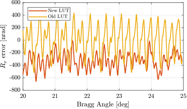
lut_new_drx   = h5read('Qutools_test_0001.h5','/34.1/instrument/xtal_111_drx_filter/data');

Comparison of the $R_x$ error for the current LUT method and the proposed one

If we zoom on the 20deg to 25deg bragg angles, we can see that the new method has much less "periodic errors" as compared to the previous one which shows some patterns.

Attocube Calibration

<<sec:dcm_attocube_lut>>

Introduction   ignore

The idea is to calibrate the periodic non-linearity of the interferometers, a known displacement must be imposed and the interferometer output compared to this displacement. This should be performed over several periods in order to characterize the error.

We here suppose that we are already in the frame of the Attocube (the fast-jack displacements are converted to Attocube displacement using the transformation matrices). We also suppose that we are at a certain Bragg angle, and that the stepper motors are not moving: only the piezoelectric actuators are used.

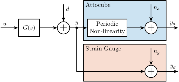
The setup is schematically with the block diagram in Figure fig:block_diagram_lut_attocube. The signals are:

• $u$: Actuator Signal (position where we wish to go)
• $d$: Disturbances affecting the signal
• $y$: Displacement of the crystal
• $y_g$: Measurement of the crystal motion by the strain gauge with some noise $n_g$
• $y_a$: Measurement of the crystal motion by the interferometer with some noise $n_a$

\definecolor{myblue}{rgb}{0, 0.447, 0.741}
\definecolor{myred}{rgb}{0.8500, 0.325, 0.098}

\begin{tikzpicture}
  \node[block] (G) at (0,0){$G(s)$};
  \node[addb, right=1 of G] (addd) {};
  \node[block, align=center, right=1 of addd] (non_linearity) {Periodic\\Non-linearity};
  \node[addb, right=1 of non_linearity] (addna) {};
  \node[addb, below=1.8 of addna] (addnsg) {};

  \draw[->] ($(G.west) + (-1.0, 0)$) node[above right]{$u$} -- (G.west);
  \draw[->] (G.east) -- (addd.west);
  \draw[->] (addd.east) -- (non_linearity.west);
  \draw[->] ($(addd.north) + (0, 1.0)$) node[below right]{$d$} -- (addd.north);
  \draw[->] (non_linearity.east) -- (addna.west);
  \draw[->] (addna.east) -- ++(1.2, 0) node[above left]{$y_a$};
  \draw[->] ($(addna.north) + (0, 1.0)$) node[below right](na){$n_a$} -- (addna.north);
  \draw[->] ($(addd.east) + (0.4, 0)$)node[branch]{} node[above]{$y$} |- (addnsg.west);
  \draw[->] (addnsg.east) -- ++(1.2, 0) node[above left]{$y_g$};
  \draw[->] ($(addnsg.north) + (0, 1.0)$) node[below right](nsg){$n_{g}$} -- (addnsg.north);

  \begin{scope}[on background layer]
    \node[fit={(non_linearity.south west) (na.north east)}, fill=myblue!20!white, draw, inner sep=6pt] (attocube) {};
    \node[fit={(non_linearity.west|-addnsg.south) (nsg.north east)}, fill=myred!20!white, draw, inner sep=6pt] (straingauge) {};
    \node[below right] at (attocube.north west) {Attocube};
    \node[below right] at (straingauge.north west) {Strain Gauge};
  \end{scope}
\end{tikzpicture}

Block Diagram schematic of the setup used to measure the periodic non-linearity of the Attocube

The problem is to estimate the periodic non-linearity of the Attocube from the imperfect measurments $y_a$ and $y_g$.

Then a Lookup Table (LUT) is build.

The wavelength of the Attocube is 1530nm, therefore the non-linearity has a period of 765nm. The amplitude of the non-linearity can vary from one unit to the other (and maybe from one experimental condition to the other). It is typically between 5nm peak to peak and 20nm peak to peak.

Simulations

We have some constrains on the way the motion is imposed and measured:

• We want the frequency content of the imposed motion to be at low frequency in order not to induce vibrations of the structure. We have to make sure the forces applied by the piezoelectric actuator only moves the crystal and not the fast jack below. Therefore, we have to move much slower than the first resonance frequency in the system.
• As both $y_a$ and $y_g$ should have rather small noise, we have to filter them with low pass filters. The cut-off frequency of the low pass filter should be high as compared to the motion (to not induce any distortion) but still reducing sufficiently the noise. Let's say we want the noise to be less than 1nm ($6 \sigma$).

Suppose we have the power spectral density (PSD) of both $n_a$ and $n_g$.

• Take the PSD of the Attocube
• Take the PSD of the strain gauge
• Using 2nd order low pass filter, estimate the required low pass filter cut-off frequency to have sufficiently low noise

Bibliography   ignore