dcm-stepper-calibration/dcm_lookup_tables.org

ESRF Double Crystal Monochromator - Lookup Tables

• Introduction
• Stepper Motors Calibration
  • Introduction
  • Schematic
  • Simulation
• Bibliography

---

This report is also available as a pdf.

---

Introduction

Stepper Motors Calibration

<<sec:dcm_stepper_lut>>

Introduction   ignore

Schematic

Simulation

In this section, we suppose that we are in the frame of one fast jack (all transformations are already done), and we wish to create a LUT for one fast jack.

Let's say with make a Bragg angle scan between 10deg and 60deg during 100s.

Fs = 10e3; % Sample Frequency [Hz]
t = 0:1/Fs:10; % Time vector [s]
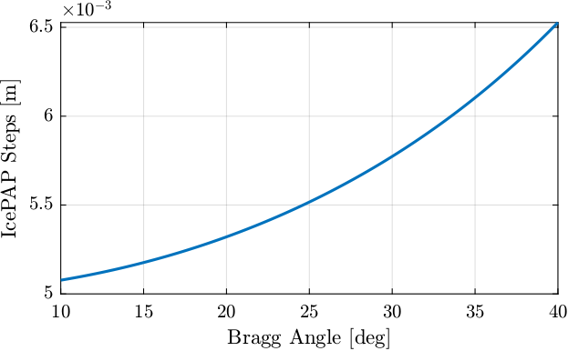
theta = linspace(10, 40, length(t)); % Bragg Angle [deg]

The IcePAP steps are following the theoretical formula:

\begin{equation} d_z = \frac{d_{\text{off}}}{2 \cos \theta} \end{equation}

with $\theta$ the bragg angle and $d_{\text{off}} = 10\,mm$.

The motion to follow is then:

perfect_motion = 10e-3./(2*cos(theta*pi/180)); % Perfect motion [m]

And the IcePAP is generated those steps:

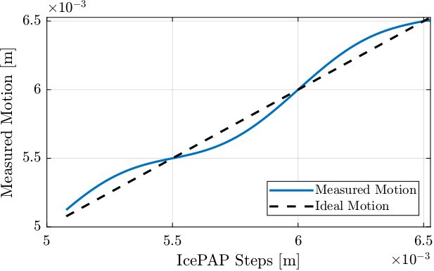
icepap_steps = perfect_motion; % IcePAP steps measured by Speedgoat [m]

IcePAP Steps as a function of the Bragg Angle

Then, we are measuring the motion of the Fast Jack using the Interferometer. The motion error is larger than in reality to be angle to see it more easily.

motion_error = 100e-6*sin(2*pi*perfect_motion/1e-3); % Error motion [m]

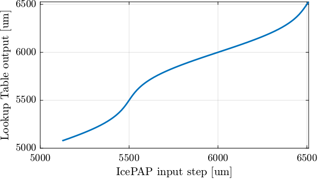
measured_motion = perfect_motion + motion_error; % Measured motion of the Fast Jack [m]

Measured motion as a function of the IcePAP Steps

Let's now compute the lookup table. For each micrometer of the IcePAP step, another step is associated that correspond to a position closer to the wanted position.

%% Get range for the LUT
% We correct only in the range of tested/measured motion
lut_range = round(1e6*min(icepap_steps)):round(1e6*max(icepap_steps)); % IcePAP steps [um]

%% Initialize the LUT
lut = zeros(size(lut_range));

%% For each um in this range
for i = 1:length(lut_range)
    % Get points indices where the measured motion is closed to the wanted one
    close_points = measured_motion > 1e-6*lut_range(i) - 500e-9 & measured_motion < 1e-6*lut_range(i) + 500e-9;
    % Get the corresponding closest IcePAP step
    lut(i) = round(1e6*mean(icepap_steps(close_points))); % [um]
end

Generated Lookup Table

The current LUT implementation is the following:

motion_error_lut = zeros(size(lut_range));
for i = 1:length(lut_range)
    % Get points indices where the icepap step is close to the wanted one
    close_points = icepap_steps > 1e-6*lut_range(i) - 500e-9 & icepap_steps < 1e-6*lut_range(i) + 500e-9;
    % Get the corresponding motion error
    motion_error_lut(i) = lut_range(i) + (lut_range(i) - round(1e6*mean(measured_motion(close_points)))); % [um]
end

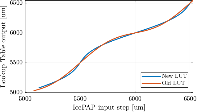
Let's compare the two Lookup Table in Figure fig:lut_comparison_two_methods.

Comparison of the two lookup tables

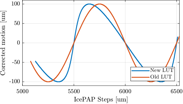
If we plot the "corrected steps" for all steps for both methods, we clearly see the difference (Figure fig:lut_correct_and_motion_error).

LUT correction and motion error as a function of the IcePAP steps

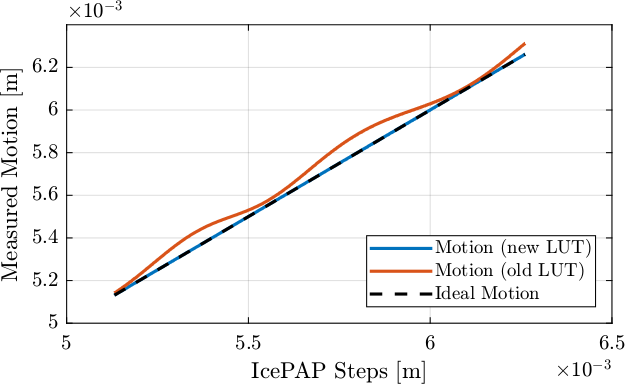
Let's now implement both LUT to see which implementation is correct.

motion_new = zeros(size(icepap_steps_output_new));
motion_old = zeros(size(icepap_steps_output_old));

for i = 1:length(icepap_steps_output_new)
    [~, i_step] = min(abs(icepap_steps_output_new(i) - 1e6*icepap_steps));
    motion_new(i) = measured_motion(i_step);

    [~, i_step] = min(abs(icepap_steps_output_old(i) - 1e6*icepap_steps));
    motion_old(i) = measured_motion(i_step);
end

Comparison of the obtained motion with new and old LUT

Bibliography   ignore