34 KiB
DCM - Dynamical Multi-Body Model
- System Kinematics
- System Identification
- Active Damping Plant (Strain gauge)
- Active Damping Plant (Force Sensors)
- HAC-LAC (IFF) architecture
- Bibliography
This report is also available as a pdf.
\clearpage
System Kinematics
Introduction ignore
Bragg Angle
%% Tested bragg angles
bragg = linspace(5, 80, 1000); % Bragg angle [deg]
d_off = 10.5e-3; % Wanted offset between x-rays [m]
%% Vertical Jack motion as a function of Bragg angle
dz = d_off./(2*cos(bragg*pi/180));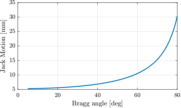
%% Required Jack stroke
ans = 1e3*(dz(end) - dz(1))
24.963
Kinematics (111 Crystal)
Introduction ignore
The reference frame is taken at the center of the 111 second crystal.
Interferometers - 111 Crystal
Three interferometers are pointed to the bottom surface of the 111 crystal.
The position of the measurement points are shown in Figure fig:sensor_111_crystal_points as well as the origin where the motion of the crystal is computed.
\begin{tikzpicture}
  % Crystal
  \draw (-15/2, -3.5/2) rectangle (15/2, 3.5/2);

  % Measurement Points
  \node[branch] (a1) at (-7,  1.5){};
  \node[branch] (a2) at ( 0, -1.5){};
  \node[branch] (a3) at ( 7,  1.5){};

  % Labels
  \node[right] at (a1) {$\mathcal{O}_1 = (-0.07, -0.015)$};
  \node[right] at (a2) {$\mathcal{O}_2 = (0,      0.015)$};
  \node[left]  at (a3) {$\mathcal{O}_3 = ( 0.07, -0.015)$};

  % Origin
  \draw[->] (0, 0) node[] -- ++(1,  0) node[right]{$x$};
  \draw[->] (0, 0) -- ++(0, -1) node[below]{$y$};
  \draw[fill, color=black] (0, 0) circle (0.05);

  \node[left] at (0,0) {$\mathcal{O}_{111}$};
\end{tikzpicture}
The inverse kinematics consisting of deriving the interferometer measurements from the motion of the crystal (see Figure fig:schematic_sensor_jacobian_inverse_kinematics):
\begin{equation} \begin{bmatrix} x_1 \\ x_2 \\ x_3 \end{bmatrix} = \bm{J}_{s,111} \begin{bmatrix} d_z \\ r_y \\ r_x \end{bmatrix} \end{equation}\begin{tikzpicture}
% Blocs
\node[block] (Js) {$\bm{J}_{s,111}$};
% Connections and labels
\draw[->] ($(Js.west)+(-1.5,0)$) node[above right]{$\begin{bmatrix} d_z \\ r_y \\ r_x \end{bmatrix}$} -- (Js.west);
\draw[->] (Js.east) -- ++(1.5, 0) node[above left]{$\begin{bmatrix} x_1 \\ x_2 \\ x_3 \end{bmatrix}$};
\end{tikzpicture}
From the Figure fig:sensor_111_crystal_points, the inverse kinematics can be solved as follow (for small motion):
\begin{equation} \bm{J}_{s,111} = \begin{bmatrix} 1 & 0.07 & -0.015 \\ 1 & 0 & 0.015 \\ 1 & -0.07 & -0.015 \end{bmatrix} \end{equation}%% Sensor Jacobian matrix for 111 crystal
J_s_111 = [1, 0.07, -0.015
1, 0, 0.015
1, -0.07, -0.015];| 1.0 | 0.07 | -0.015 |
| 1.0 | 0.0 | 0.015 |
| 1.0 | -0.07 | -0.015 |
The forward kinematics is solved by inverting the Jacobian matrix (see Figure fig:schematic_sensor_jacobian_forward_kinematics).
\begin{equation} \begin{bmatrix} d_z \\ r_y \\ r_x \end{bmatrix} = \bm{J}_{s,111}^{-1} \begin{bmatrix} x_1 \\ x_2 \\ x_3 \end{bmatrix} \end{equation}\begin{tikzpicture}
% Blocs
\node[block] (Js_inv) {$\bm{J}_{s,111}^{-1}$};
% Connections and labels
\draw[->] ($(Js_inv.west)+(-1.5,0)$) node[above right]{$\begin{bmatrix} x_1 \\ x_2 \\ x_3 \end{bmatrix}$} -- (Js_inv.west);
\draw[->] (Js_inv.east) -- ++(1.5, 0) node[above left]{$\begin{bmatrix} d_z \\ r_y \\ r_x \end{bmatrix}$};
\end{tikzpicture}
| 0.25 | 0.5 | 0.25 |
| 7.14 | 0.0 | -7.14 |
| -16.67 | 33.33 | -16.67 |
Piezo - 111 Crystal
The location of the actuators with respect with the center of the 111 second crystal are shown in Figure fig:actuator_jacobian_111_points.
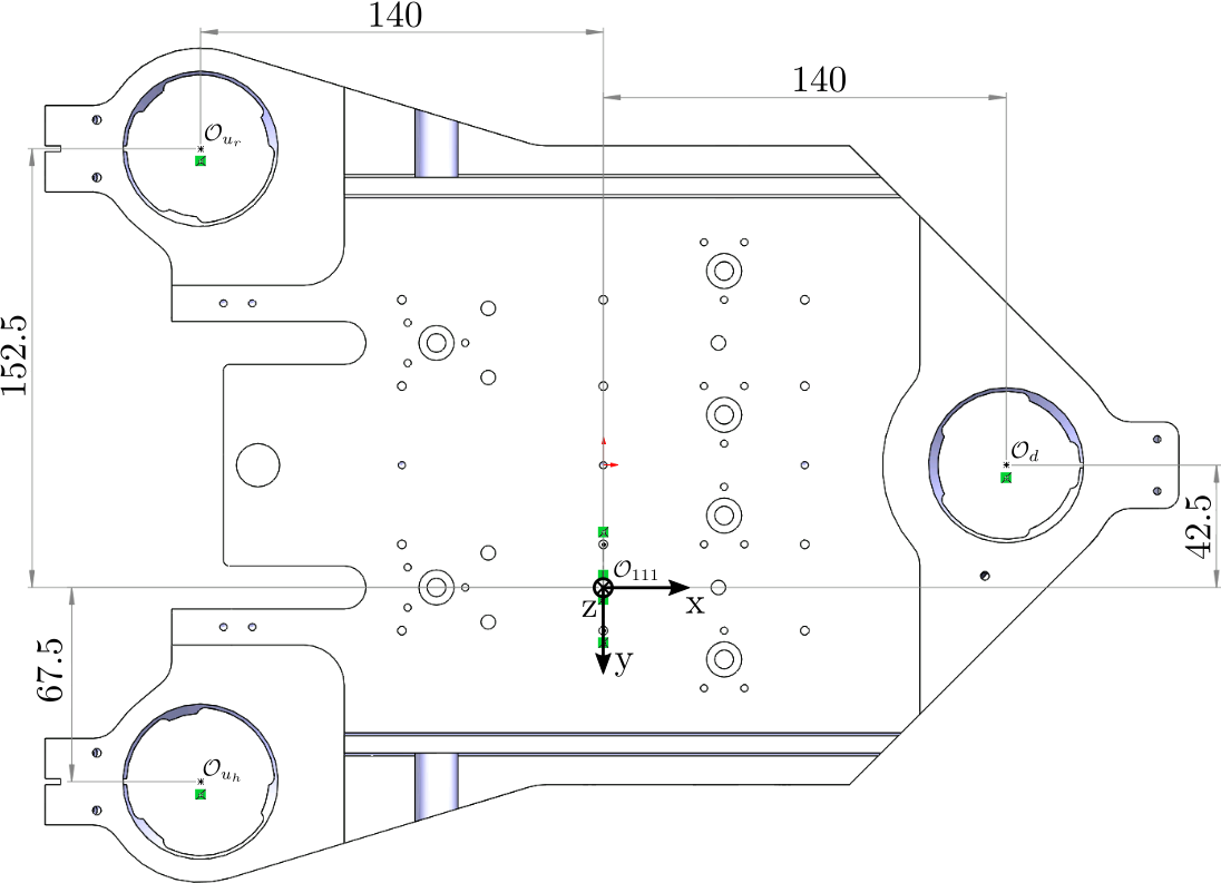
Inverse Kinematics consist of deriving the axial (z) motion of the 3 actuators from the motion of the crystal's center.
\begin{equation} \begin{bmatrix} d_{u_r} \\ d_{u_h} \\ d_{d} \end{bmatrix} = \bm{J}_{a,111} \begin{bmatrix} d_z \\ r_y \\ r_x \end{bmatrix} \end{equation}\begin{tikzpicture}
% Blocs
\node[block] (Ja) {$\bm{J}_{a,111}$};
% Connections and labels
\draw[->] ($(Ja.west)+(-1.5,0)$) node[above right]{$\begin{bmatrix} d_z \\ r_y \\ r_x \end{bmatrix}$} -- (Ja.west);
\draw[->] (Ja.east) -- ++(1.5, 0) node[above left]{$\begin{bmatrix} d_{u_r} \\ d_{u_h} \\ d_d \end{bmatrix}$};
\end{tikzpicture}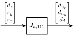
Based on the geometry in Figure fig:actuator_jacobian_111_points, we obtain:
\begin{equation} \bm{J}_{a,111} = \begin{bmatrix} 1 & 0.14 & -0.1525 \\ 1 & 0.14 & 0.0675 \\ 1 & -0.14 & -0.0425 \end{bmatrix} \end{equation}%% Actuator Jacobian - 111 crystal
J_a_111 = [1, 0.14, -0.1525
1, 0.14, 0.0675
1, -0.14, -0.0425];| 1.0 | 0.14 | -0.1525 |
| 1.0 | 0.14 | 0.0675 |
| 1.0 | -0.14 | -0.0425 |
The forward Kinematics is solved by inverting the Jacobian matrix:
\begin{equation} \begin{bmatrix} d_z \\ r_y \\ r_x \end{bmatrix} = \bm{J}_{a,111}^{-1} \begin{bmatrix} d_{u_r} \\ d_{u_h} \\ d_{d} \end{bmatrix} \end{equation}\begin{tikzpicture}
% Blocs
\node[block] (Ja_inv) {$\bm{J}_{a,111}^{-1}$};
% Connections and labels
\draw[->] ($(Ja_inv.west)+(-1.5,0)$) node[above right]{$\begin{bmatrix} d_{u_r} \\ d_{u_h} \\ d_d \end{bmatrix}$} -- (Ja_inv.west);
\draw[->] (Ja_inv.east) -- ++(1.5, 0) node[above left]{$\begin{bmatrix} d_z \\ r_y \\ r_x \end{bmatrix}$};
\end{tikzpicture}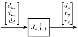
| 0.0568 | 0.4432 | 0.5 |
| 1.7857 | 1.7857 | -3.5714 |
| -4.5455 | 4.5455 | 0.0 |
Save Kinematics
save('mat/dcm_kinematics.mat', 'J_a_111', 'J_s_111')System Identification
Introduction ignore
Identification
Let's considered the system $\bm{G}(s)$ with:
- 3 inputs: force applied to the 3 fast jacks
- 3 outputs: measured displacement by the 3 interferometers pointing at the 111 second crystal
It is schematically shown in Figure fig:schematic_system_inputs_outputs.
\begin{tikzpicture}
  % Blocs
  \node[block] (G) {$\bm{G}(s)$};

  % Connections and labels
  \draw[->] ($(G.west)+(-1.5,0)$) node[above right]{$\begin{bmatrix} u_{u_r} \\ u_{u_h} \\ u_d \end{bmatrix}$} -- (G.west);
  \draw[->] (G.east)  -- ++(1.5, 0) node[above left]{$\begin{bmatrix} x_1 \\ x_2 \\ x_3 \end{bmatrix}$};
\end{tikzpicture}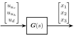
The system is identified from the Simscape model.
%% Input/Output definition
clear io; io_i = 1;

%% Inputs
% Control Input {3x1} [N]
io(io_i) = linio([mdl, '/control_system'], 1, 'openinput');  io_i = io_i + 1;

%% Outputs
% Interferometers {3x1} [m]
io(io_i) = linio([mdl, '/DCM'], 1, 'openoutput'); io_i = io_i + 1;
%% Extraction of the dynamics
G = linearize(mdl, io);size(G)size(G) State-space model with 3 outputs, 3 inputs, and 24 states.
Plant in the frame of the fastjacks
load('mat/dcm_kinematics.mat');Using the forward and inverse kinematics, we can computed the dynamics from piezo forces to axial motion of the 3 fastjacks (see Figure fig:schematic_jacobian_frame_fastjack).
\begin{tikzpicture}
  % Blocs
  \node[block] (G) {$\bm{G}(s)$};
  \node[block, right=1.5 of G] (Js) {$\bm{J}_{s}^{-1}$};
  \node[block, right=1.5 of Js] (Ja) {$\bm{J}_{a}$};

  % Connections and labels
  \draw[->] ($(G.west)+(-1.5,0)$) node[above right]{$\begin{bmatrix} u_{u_r} \\ u_{u_h} \\ u_d \end{bmatrix}$} -- (G.west);
  \draw[->] (G.east)  -- node[midway, above]{$\begin{bmatrix} x_1 \\ x_2 \\ x_3 \end{bmatrix}$} (Js.west);
  \draw[->] (Js.east) -- node[midway, above]{$\begin{bmatrix} d_z \\ r_y \\ r_x \end{bmatrix}$} (Ja.west);
  \draw[->] (Ja.east) -- ++(1.5, 0) node[above left]{$\begin{bmatrix} d_{u_r} \\ d_{u_h} \\ d_{d} \end{bmatrix}$};

  \begin{scope}[on background layer]
    \node[fit={(G.south west) ($(Ja.east)+(0, 1.4)$)}, fill=black!20!white, draw, inner sep=6pt] (system) {};
    \node[above] at (system.north) {$\bm{G}_{\text{fj}}(s)$};
  \end{scope}
\end{tikzpicture}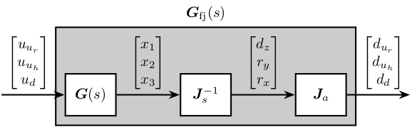
%% Compute the system in the frame of the fastjacks
G_pz = J_a_111*inv(J_s_111)*G;
The DC gain of the new system shows that the system is well decoupled at low frequency.
dcgain(G_pz)| 4.4407e-09 | 2.7656e-12 | 1.0132e-12 |
| 2.7656e-12 | 4.4407e-09 | 1.0132e-12 |
| 1.0109e-12 | 1.0109e-12 | 4.4424e-09 |
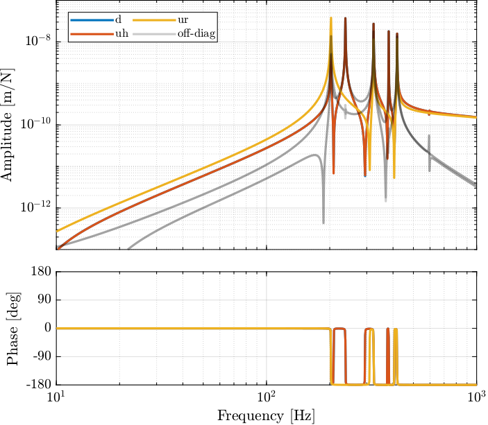
The bode plot of $\bm{G}_{\text{fj}}(s)$ is shown in Figure fig:bode_plot_plant_fj.
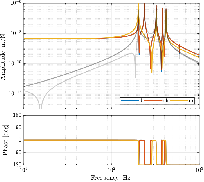
Computing the system in the frame of the fastjack gives good decoupling at low frequency (until the first resonance of the system).
Plant in the frame of the crystal
\begin{tikzpicture}
  % Blocs
  \node[block] (G) {$\bm{G}(s)$};
  \node[block, left=1.5 of G] (Ja) {$\bm{J}_{a}^{-T}$};
  \node[block, right=1.5 of G] (Js) {$\bm{J}_{s}^{-1}$};

  % Connections and labels
  \draw[->] ($(Ja.west)+(-1.5,0)$) node[above right]{$\begin{bmatrix} \mathcal{F}_{z} \\ \mathcal{M}_{y} \\ \mathcal{M}_{x} \end{bmatrix}$} -- (Ja.west);
  \draw[->] (Ja.east)  -- node[midway, above]{$\begin{bmatrix} u_{u_r} \\ u_{u_h} \\ u_d \end{bmatrix}$} (G.west);
  \draw[->] (G.east) -- node[midway, above]{$\begin{bmatrix} x_1 \\ x_2 \\ x_3 \end{bmatrix}$} (Js.west);
  \draw[->] (Js.east) -- ++(1.5, 0) node[above left]{$\begin{bmatrix} d_z \\ r_y \\ r_x \end{bmatrix}$};

  \begin{scope}[on background layer]
    \node[fit={(Ja.south west) ($(Js.east)+(0, 1.4)$)}, fill=black!20!white, draw, inner sep=6pt] (system) {};
    \node[above] at (system.north) {$\bm{G}_{\text{cr}}(s)$};
  \end{scope}
\end{tikzpicture}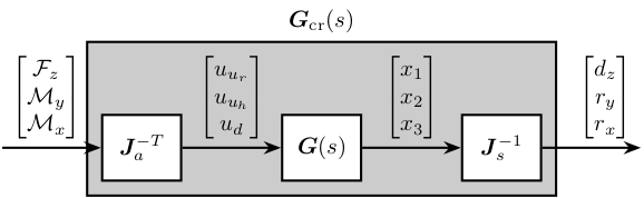
G_mr = inv(J_s_111)*G*inv(J_a_111');dcgain(G_mr)| 1.9978e-09 | 3.9657e-09 | 7.7944e-09 |
| 3.9656e-09 | 8.4979e-08 | -1.5135e-17 |
| 7.7944e-09 | -3.9252e-17 | 1.834e-07 |
This results in a coupled system. The main reason is that, as we map forces to the center of the 111 crystal and not at the center of mass/stiffness of the moving part, vertical forces will induce rotation and torques will induce vertical motion.
Active Damping Plant (Strain gauge)
Introduction ignore
In this section, we wish to see whether if strain gauges fixed to the piezoelectric actuator can be used for active damping.
Identification
%% Input/Output definition
clear io; io_i = 1;

%% Inputs
% Control Input {3x1} [N]
io(io_i) = linio([mdl, '/u'], 1, 'openinput');  io_i = io_i + 1;
% % Stepper Displacement {3x1} [m]
% io(io_i) = linio([mdl, '/d'], 1, 'openinput');  io_i = io_i + 1;

%% Outputs
% Strain Gauges {3x1} [m]
io(io_i) = linio([mdl, '/sg'], 1, 'openoutput'); io_i = io_i + 1;
%% Extraction of the dynamics
G_sg = linearize(mdl, io);dcgain(G_sg)| -1.4113e-13 | 1.0339e-13 | 3.774e-14 |
| 1.0339e-13 | -1.4113e-13 | 3.774e-14 |
| 3.7792e-14 | 3.7792e-14 | -7.5585e-14 |
Active Damping Plant (Force Sensors)
Introduction ignore
Force sensors are added above the piezoelectric actuators. They can consists of a simple piezoelectric ceramic stack. See for instance cite:fleming10_integ_strain_force_feedb_high.
Identification
%% Input/Output definition
clear io; io_i = 1;

%% Inputs
% Control Input {3x1} [N]
io(io_i) = linio([mdl, '/control_system'], 1, 'openinput');  io_i = io_i + 1;

%% Outputs
% Force Sensor {3x1} [m]
io(io_i) = linio([mdl, '/DCM'], 3, 'openoutput'); io_i = io_i + 1;
%% Extraction of the dynamics
G_fs = linearize(mdl, io);dcgain(G_fs)| -1.4113e-13 | 1.0339e-13 | 3.774e-14 |
| 1.0339e-13 | -1.4113e-13 | 3.774e-14 |
| 3.7792e-14 | 3.7792e-14 | -7.5585e-14 |
Controller - Root Locus
Kiff_g1 = eye(3)*1/(1 + s/2/pi/20);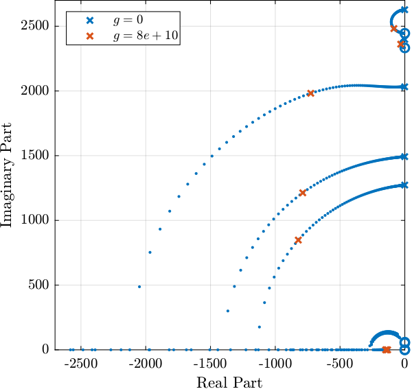
%% Integral Force Feedback Controller
Kiff = g*Kiff_g1;
Damped Plant
%% Input/Output definition
clear io; io_i = 1;

%% Inputs
% Control Input {3x1} [N]
io(io_i) = linio([mdl, '/control_system'], 1, 'input');  io_i = io_i + 1;

%% Outputs
% Force Sensor {3x1} [m]
io(io_i) = linio([mdl, '/DCM'], 1, 'openoutput'); io_i = io_i + 1;
%% DCM Kinematics
load('mat/dcm_kinematics.mat');%% Identification of the Open Loop plant
controller.type = 0; % Open Loop
G_ol = J_a_111*inv(J_s_111)*linearize(mdl, io);
G_ol.InputName = {'u_ur', 'u_uh', 'u_d'};
G_ol.OutputName = {'d_ur', 'd_uh', 'd_d'};%% Identification of the damped plant with IFF
controller.type = 1; % IFF
G_dp = J_a_111*inv(J_s_111)*linearize(mdl, io);
G_dp.InputName = {'u_ur', 'u_uh', 'u_d'};
G_dp.OutputName = {'d_ur', 'd_uh', 'd_d'};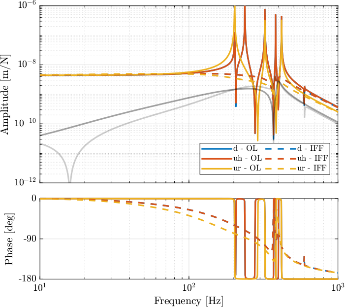
The Integral Force Feedback control strategy is very effective in damping the suspension modes of the DCM.
Save
save('mat/Kiff.mat', 'Kiff');