6.7 KiB
Attocube - Test Bench
Estimation of the Spectral Density of the Attocube Noise
Long and Slow measurement
The first measurement was made during ~17 hours with a sampling time of $T_s = 0.1\,s$.
  load('./mat/long_test2.mat', 'x', 't')
  Ts = 0.1; % [s]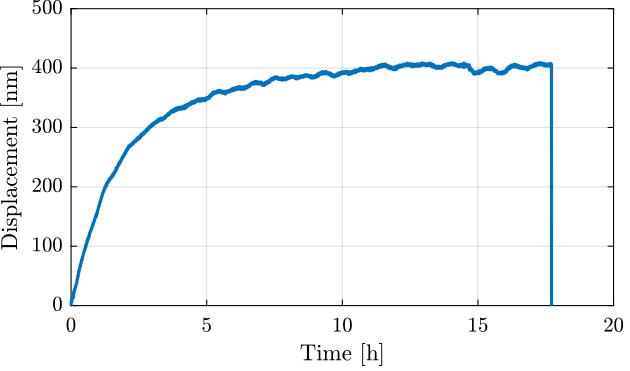
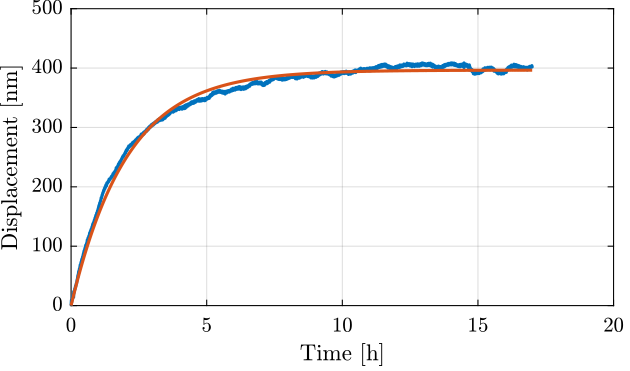
Let's fit the data with a step response to a first order low pass filter (Figure fig:long_meas_time_domain_fit).
  f = @(b,x) b(1)*(1 - exp(-x/b(2)));

  y_cur = x(t < 17*60*60);
  t_cur = t(t < 17*60*60);

  nrmrsd = @(b) norm(y_cur - f(b,t_cur)); % Residual Norm Cost Function
  B0 = [400e-9, 2*60*60];                        % Choose Appropriate Initial Estimates
  [B,rnrm] = fminsearch(nrmrsd, B0);     % Estimate Parameters ‘B’
The corresponding time constant is (in [h]):
2.0576
We can see in Figure fig:long_meas_time_domain_full that there is a transient period where the measured displacement experiences some drifts.
This is probably due to thermal effects.
We only select the data between t1 and t2.
The obtained displacement is shown in Figure fig:long_meas_time_domain_zoom.
  t1 = 11; t2 = 17; % [h]

  x = x(t > t1*60*60 & t < t2*60*60);
  x = x - mean(x);
  t = t(t > t1*60*60 & t < t2*60*60);
  t = t - t(1);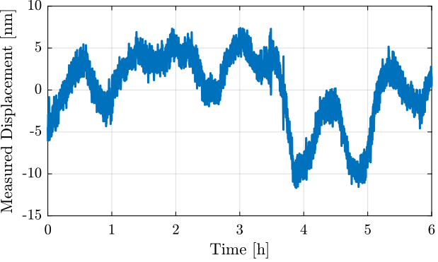
The Power Spectral Density of the measured displacement is computed
  win = hann(ceil(length(x)/20));
  [p_1, f_1] = pwelch(x, win, [], [], 1/Ts);
Short and Fast measurement
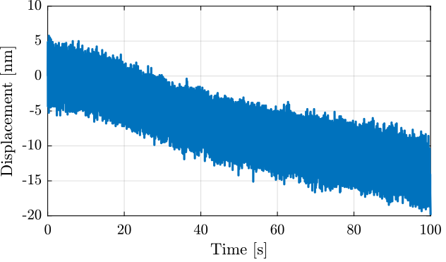
An second measurement is done in order to estimate the high frequency noise of the interferometer. The measurement is done with a sampling time of $T_s = 0.1\,ms$ and a duration of ~100s.
  load('./mat/test.mat', 'x', 't')
  Ts = 1e-4; % [s]
The time domain measurement is shown in Figure fig:short_meas_time_domain.
The Power Spectral Density of the measured displacement is computed
win = hann(ceil(length(x)/20));
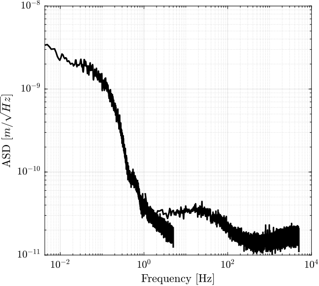
[p_2, f_2] = pwelch(x, win, [], [], 1/Ts);Obtained Amplitude Spectral Density of the measured displacement
The computed ASD of the two measurements are combined in Figure fig:psd_combined.