Flexible Joint - Test Bench

1. Flexible Joints - Requirements
2. Test Bench Description
3. Agreement between the probe and the encoder
- 3.1. Setup
- 3.2. Results
4. Measurement of the Millimar 1318 probe stiffness
- 4.1. Results
5. Experimental measurement

This report is also available as a pdf.

1 Flexible Joints - Requirements

	Specification
Axial Stiffness	> 200 [N/um]
Shear Stiffness	> 1 [N/um]
Bending Stiffness	< 100 [Nm/rad]
Torsion Stiffness	< 500 [Nm/rad]
Bending Stroke	> 1 [mrad]
Torsion Stroke	> 5 [urad]

2 Test Bench Description

The main characteristic of the flexible joint that we want to measure is its bending stiffness \(k_{R_x} \approx k_{R_y}\).

To do so, a test bench is used. Specifications of the test bench to precisely measure the bending stiffness are described in this section.

The basic idea is to measured the angular deflection of the flexible joint as a function of the applied torque.

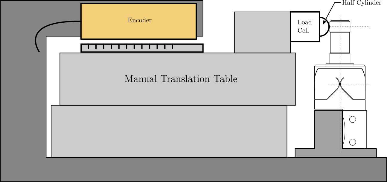
Figure 1: Schematic of the test bench to measure the bending stiffness of the flexible joints

2.1 Flexible joint Geometry

The flexible joint used for the Nano-Hexapod is shown in Figure 2. Its bending stiffness is foreseen to be \(k_{R_y}\approx 20\,\frac{Nm}{rad}\) and its stroke \(\theta_{y,\text{max}}\approx 20\,mrad\).

Figure 2: Geometry of the flexible joint

The height between the flexible point (center of the joint) and the point where external forces are applied is \(h = 20\,mm\).

Let’s define the parameters on Matlab.

  kRx = 20; % Bending Stiffness [Nm/rad]
  Rxmax = 20e-3; % Bending Stroke [rad]
  h = 20e-3; % Height [m]

2.2 Required external applied force

The bending \(\theta_y\) of the flexible joint due to the force \(F_x\) is:

\begin{equation} \theta_y = \frac{M_y}{k_{R_y}} = \frac{F_x h}{k_{R_y}} \end{equation}

Therefore, the applied force to test the full range of the flexible joint is:

\begin{equation} F_{x,\text{max}} = \frac{k_{R_y} \theta_{y,\text{max}}}{h} \end{equation}

  Fxmax = kRx*Rxmax/h; % Force to induce maximum stroke [N]

And we obtain:

\begin{equation} F_{max} = 20.0\, [N] \end{equation}

The measurement range of the force sensor should then be higher than \(20\,N\).

2.3 Required actuator stroke and sensors range

The flexible joint is designed to allow a bending motion of \(\pm 20\,mrad\). The corresponding actuator stroke to impose such motion is:

\[ d_{x,\text{max}} = h \tan(R_{x,\text{max}}) \]

  dxmax = h*tan(Rxmax);

\begin{equation} d_{max} = 0.4\, [mm] \end{equation}

In order to test the full range of the flexible joint, the stroke of the actuator should be higher than \(0.4\,mm\). The measurement range of the displacement sensor should also be higher than \(0.4\,mm\).

2.4 First try with the APA95ML

The APA95ML as a stroke of \(100\,\mu m\) and the encoder in parallel can easily measure the required stroke.

Suppose the full stroke of the APA can be used to bend the flexible joint (ideal case), the measured force will be:

  Fxmax = kRx*100e-6/h^2; % Force at maximum stroke [N]

\begin{equation} F_{max} = 5.0\, [N] \end{equation}

And the tested angular range is:

  Rmax = tan(100e-6/h);

\begin{equation} \theta_{max} = 5.0\, [mrad] \end{equation}

2.5 Test Bench

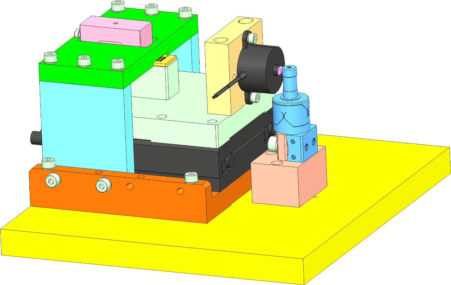
Figure 3: Schematic of the test bench to measure the bending stiffness of the flexible joints

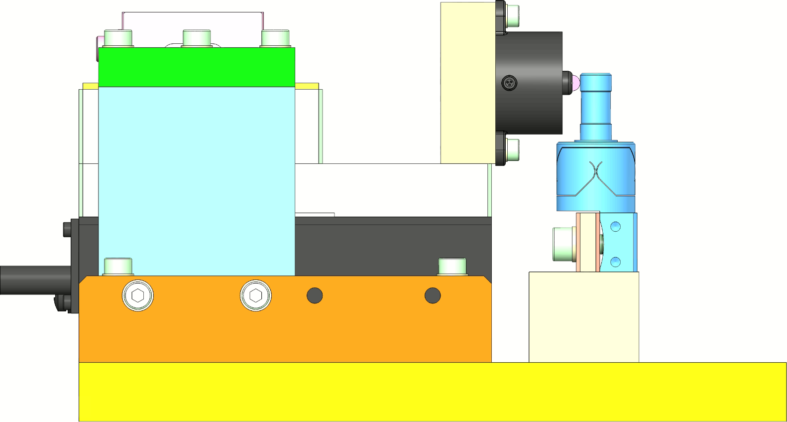
Figure 4: Schematic of the test bench to measure the bending stiffness of the flexible joints

Translation Stage: V-408
Load Cells: FC2231-0000-0010-L and XFL212R
Encoder: Renishaw Resolute 1nm
Displacement Probe: Millimar C1216 electronics and Millimar 1318 probe

3 Agreement between the probe and the encoder

3.1 Setup

The measurement setup is made such that the probe measured the translation table displacement. It should then measure the same displacement as the encoder. Using this setup, we should be able to compare the probe and the encoder.

3.2 Results

Let’s load the measurements.

load('meas_probe_against_encoder.mat', 't', 'd', 'dp', 'F')

The time domain measured displacement by the probe and by the encoder is shown in Figure 5.

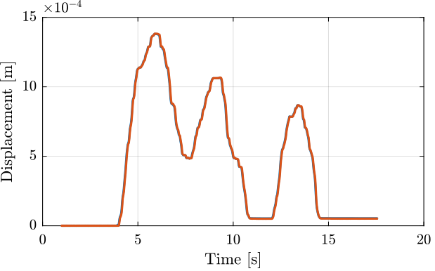
Figure 5: Time domain measurement

If we zoom, we see that there is some delay between the encoder and the probe (Figure 6).

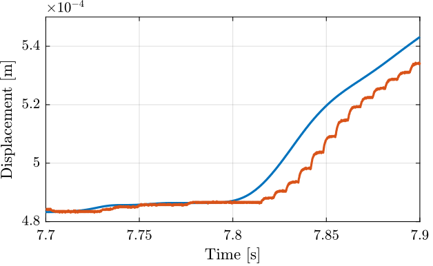
Figure 6: Time domain measurement (Zoom)

This delay is estimated using the finddelay command.

The time delay is approximately 15.8 [ms]

The measured mismatch between the encoder and the probe with and without compensating for the time delay are shown in Figure 7.

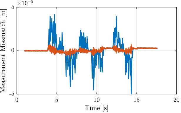
Figure 7: Measurement mismatch, with and without delay compensation

Finally, the displacement of the probe is shown as a function of the displacement of the encoder and a linear fit is made (Figure 8).

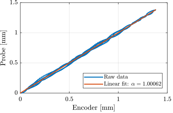
Figure 8: Measured displacement by the probe as a function of the measured displacement by the encoder

From the measurement, it is shown that the probe is well calibrated. However, there is some time delay of tens of milliseconds that could induce some measurement errors.

4 Measurement of the Millimar 1318 probe stiffness

Translation Stage: V-408
Load Cell: FC2231-0000-0010-L
Encoder: Renishaw Resolute 1nm
Displacement Probe: Millimar C1216 electronics and Millimar 1318 probe

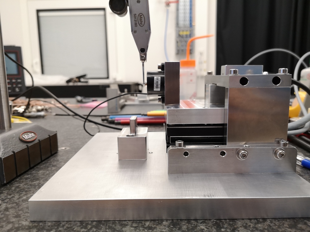
Figure 9: Setup - Side View

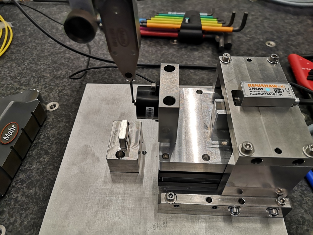
Figure 10: Setup - Top View

4.1 Results

Let’s load the measurement results.

load('meas_stiff_probe.mat', 't', 'd', 'dp', 'F')

The time domain measured force and displacement are shown in Figure 11.

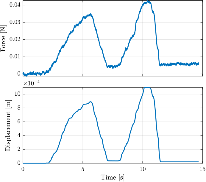
Figure 11: Time domain measurements

Now we can estimate the stiffness with a linear fit.

Stiffness is 0.039 [N/mm]

This is very close to the 0.04 [N/mm] written in the Millimar 1318 probe datasheet.

And compare the linear fit with the raw measurement data (Figure 12).

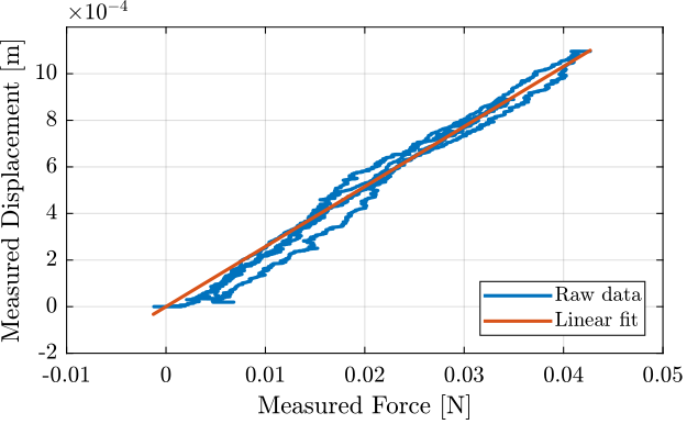
Figure 12: Measured displacement as a function of the measured force. Raw data and linear fit

The Millimar 1318 probe has a stiffness of \(\approx 0.04\,[N/mm]\).