SVD Control

1. Gravimeter - Simscape Model
2. Gravimeter - Functions
- 2.1. align
- 2.2. pzmap_testCL
3. Stewart Platform - Simscape Model
4. Stewart Platform - Analytical Model

1 Gravimeter - Simscape Model

1.1 Introduction

Figure 1: Model of the gravimeter

1.2 Simscape Model - Parameters

open('gravimeter.slx')

Parameters

l  = 1.0; % Length of the mass [m]
la = 0.5; % Position of Act. [m]

h  = 3.4; % Height of the mass [m]
ha = 1.7; % Position of Act. [m]

m = 400; % Mass [kg]
I = 115; % Inertia [kg m^2]

k = 15e3; % Actuator Stiffness [N/m]
c = 0.03; % Actuator Damping [N/(m/s)]

deq = 0.2; % Length of the actuators [m]

g = 0; % Gravity [m/s2]

1.3 System Identification - Without Gravity

%% Name of the Simulink File
mdl = 'gravimeter';

%% Input/Output definition
clear io; io_i = 1;
io(io_i) = linio([mdl, '/F1'], 1, 'openinput');  io_i = io_i + 1;
io(io_i) = linio([mdl, '/F2'], 1, 'openinput');  io_i = io_i + 1;
io(io_i) = linio([mdl, '/F3'], 1, 'openinput');  io_i = io_i + 1;
io(io_i) = linio([mdl, '/Acc_side'], 1, 'openoutput'); io_i = io_i + 1;
io(io_i) = linio([mdl, '/Acc_side'], 2, 'openoutput'); io_i = io_i + 1;
io(io_i) = linio([mdl, '/Acc_top'], 1, 'openoutput'); io_i = io_i + 1;
io(io_i) = linio([mdl, '/Acc_top'], 2, 'openoutput'); io_i = io_i + 1;

G = linearize(mdl, io);
G.InputName  = {'F1', 'F2', 'F3'};
G.OutputName = {'Ax1', 'Az1', 'Ax2', 'Az2'};

pole(G)
ans =
      -0.000473481142385795 +      21.7596190728632i
      -0.000473481142385795 -      21.7596190728632i
      -7.49842879459172e-05 +       8.6593576906982i
      -7.49842879459172e-05 -       8.6593576906982i
       -5.1538686792578e-06 +      2.27025295182756i
       -5.1538686792578e-06 -      2.27025295182756i

The plant as 6 states as expected (2 translations + 1 rotation)

size(G)

State-space model with 4 outputs, 3 inputs, and 6 states.

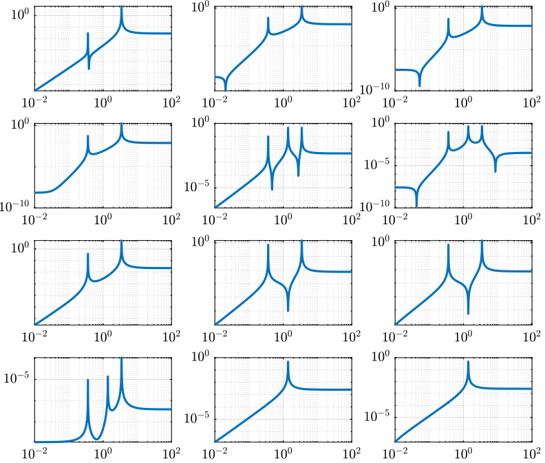
Figure 2: Open Loop Transfer Function from 3 Actuators to 4 Accelerometers

1.4 System Identification - With Gravity

g = 9.80665; % Gravity [m/s2]

Gg = linearize(mdl, io);
Gg.InputName  = {'F1', 'F2', 'F3'};
Gg.OutputName = {'Ax1', 'Az1', 'Ax2', 'Az2'};

We can now see that the system is unstable due to gravity.

pole(Gg)
ans =
          -10.9848275341252 +                     0i
           10.9838836405201 +                     0i
      -7.49855379478109e-05 +      8.65962885770051i
      -7.49855379478109e-05 -      8.65962885770051i
      -6.68819548733559e-06 +     0.832960422243848i
      -6.68819548733559e-06 -     0.832960422243848i

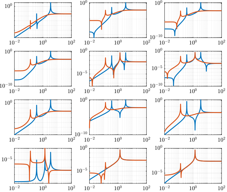
Figure 3: Open Loop Transfer Function from 3 Actuators to 4 Accelerometers with an without gravity

1.5 Analytical Model

1.5.1 Parameters

Bode options.

P = bodeoptions;
P.FreqUnits = 'Hz';
P.MagUnits = 'abs';
P.MagScale = 'log';
P.Grid = 'on';
P.PhaseWrapping = 'on';
P.Title.FontSize = 14;
P.XLabel.FontSize = 14;
P.YLabel.FontSize = 14;
P.TickLabel.FontSize = 12;
P.Xlim = [1e-1,1e2];
P.MagLowerLimMode = 'manual';
P.MagLowerLim= 1e-3;

Frequency vector.

w = 2*pi*logspace(-1,2,1000); % [rad/s]

1.5.2 Generation of the State Space Model

Mass matrix

M = [m 0 0
     0 m 0
     0 0 I];

Jacobian of the bottom sensor

Js1 = [1 0  h/2
       0 1 -l/2];

Jacobian of the top sensor

Js2 = [1 0 -h/2
       0 1  0];

Jacobian of the actuators

Ja = [1 0  ha   % Left horizontal actuator
      0 1 -la   % Left vertical actuator
      0 1  la]; % Right vertical actuator
Jta = Ja';

Stiffness and Damping matrices

K = k*Jta*Ja;
C = c*Jta*Ja;

State Space Matrices

E = [1 0 0
     0 1 0
     0 0 1]; %projecting ground motion in the directions of the legs

AA = [zeros(3) eye(3)
      -M\K -M\C];

BB = [zeros(3,6)
      M\Jta M\(k*Jta*E)];

CC = [[Js1;Js2] zeros(4,3);
      zeros(2,6)
      (Js1+Js2)./2 zeros(2,3)
      (Js1-Js2)./2 zeros(2,3)
      (Js1-Js2)./(2*h) zeros(2,3)];

DD = [zeros(4,6)
      zeros(2,3) eye(2,3)
      zeros(6,6)];

State Space model:

Input = three actuators and three ground motions
Output = the bottom sensor; the top sensor; the ground motion; the half sum; the half difference; the rotation

system_dec = ss(AA,BB,CC,DD);

size(system_dec)

State-space model with 12 outputs, 6 inputs, and 6 states.

1.5.3 Comparison with the Simscape Model

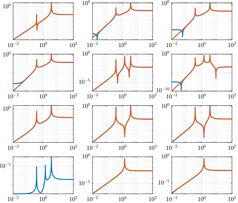
Figure 4: Comparison of the analytical and the Simscape models

1.5.4 Analysis

% figure
% bode(system_dec,P);
% return

%% svd decomposition
% system_dec_freq = freqresp(system_dec,w);
% S = zeros(3,length(w));
% for m = 1:length(w)
%     S(:,m) = svd(system_dec_freq(1:4,1:3,m));
% end
% figure
% loglog(w./(2*pi), S);hold on;
% % loglog(w./(2*pi), abs(Val(1,:)),w./(2*pi), abs(Val(2,:)),w./(2*pi), abs(Val(3,:)));
% xlabel('Frequency [Hz]');ylabel('Singular Value [-]');
% legend('\sigma_1','\sigma_2','\sigma_3');%,'\sigma_4','\sigma_5','\sigma_6');
% ylim([1e-8 1e-2]);
%
% %condition number
% figure
% loglog(w./(2*pi), S(1,:)./S(3,:));hold on;
% % loglog(w./(2*pi), abs(Val(1,:)),w./(2*pi), abs(Val(2,:)),w./(2*pi), abs(Val(3,:)));
% xlabel('Frequency [Hz]');ylabel('Condition number [-]');
% % legend('\sigma_1','\sigma_2','\sigma_3');%,'\sigma_4','\sigma_5','\sigma_6');
%
% %performance indicator
% system_dec_svd = freqresp(system_dec(1:4,1:3),2*pi*10);
% [U,S,V] = svd(system_dec_svd);
% H_svd_OL = -eye(3,4);%-[zpk(-2*pi*10,-2*pi*40,40/10) 0 0 0; 0 10*zpk(-2*pi*40,-2*pi*200,40/200) 0 0; 0 0 zpk(-2*pi*2,-2*pi*10,10/2) 0];% - eye(3,4);%
% H_svd = pinv(V')*H_svd_OL*pinv(U);
% % system_dec_control_svd_ = feedback(system_dec,g*pinv(V')*H*pinv(U));
%
% OL_dec = g_svd*H_svd*system_dec(1:4,1:3);
% OL_freq = freqresp(OL_dec,w); % OL = G*H
% CL_system = feedback(eye(3),-g_svd*H_svd*system_dec(1:4,1:3));
% CL_freq = freqresp(CL_system,w); % CL = (1+G*H)^-1
% % CL_system_2 = feedback(system_dec,H);
% % CL_freq_2 = freqresp(CL_system_2,w); % CL = G/(1+G*H)
% for i = 1:size(w,2)
%     OL(:,i) = svd(OL_freq(:,:,i));
%     CL (:,i) = svd(CL_freq(:,:,i));
%     %CL2 (:,i) = svd(CL_freq_2(:,:,i));
% end
%
% un = ones(1,length(w));
% figure
% loglog(w./(2*pi),OL(3,:)+1,'k',w./(2*pi),OL(3,:)-1,'b',w./(2*pi),1./CL(1,:),'r--',w./(2*pi),un,'k:');hold on;%
% % loglog(w./(2*pi), 1./(CL(2,:)),w./(2*pi), 1./(CL(3,:)));
% % semilogx(w./(2*pi), 1./(CL2(1,:)),w./(2*pi), 1./(CL2(2,:)),w./(2*pi), 1./(CL2(3,:)));
% xlabel('Frequency [Hz]');ylabel('Singular Value [-]');
% legend('GH \sigma_{inf} +1 ','GH \sigma_{inf} -1','S 1/\sigma_{sup}');%,'\lambda_1','\lambda_2','\lambda_3');
%
% figure
% loglog(w./(2*pi),OL(1,:)+1,'k',w./(2*pi),OL(1,:)-1,'b',w./(2*pi),1./CL(3,:),'r--',w./(2*pi),un,'k:');hold on;%
% % loglog(w./(2*pi), 1./(CL(2,:)),w./(2*pi), 1./(CL(3,:)));
% % semilogx(w./(2*pi), 1./(CL2(1,:)),w./(2*pi), 1./(CL2(2,:)),w./(2*pi), 1./(CL2(3,:)));
% xlabel('Frequency [Hz]');ylabel('Singular Value [-]');
% legend('GH \sigma_{sup} +1 ','GH \sigma_{sup} -1','S 1/\sigma_{inf}');%,'\lambda_1','\lambda_2','\lambda_3');

1.5.5 Control Section

system_dec_10Hz = freqresp(system_dec,2*pi*10);
system_dec_0Hz = freqresp(system_dec,0);

system_decReal_10Hz = pinv(align(system_dec_10Hz));
[Ureal,Sreal,Vreal] = svd(system_decReal_10Hz(1:4,1:3));
normalizationMatrixReal = abs(pinv(Ureal)*system_dec_0Hz(1:4,1:3)*pinv(Vreal'));

[U,S,V] = svd(system_dec_10Hz(1:4,1:3));
normalizationMatrix = abs(pinv(U)*system_dec_0Hz(1:4,1:3)*pinv(V'));

H_dec = ([zpk(-2*pi*5,-2*pi*30,30/5) 0 0 0
          0 zpk(-2*pi*4,-2*pi*20,20/4) 0 0
          0 0 0 zpk(-2*pi,-2*pi*10,10)]);
H_cen_OL = [zpk(-2*pi,-2*pi*10,10) 0 0; 0 zpk(-2*pi,-2*pi*10,10) 0;
            0 0 zpk(-2*pi*5,-2*pi*30,30/5)];
H_cen = pinv(Jta)*H_cen_OL*pinv([Js1; Js2]);
% H_svd_OL = -[1/normalizationMatrix(1,1) 0 0 0
%     0 1/normalizationMatrix(2,2) 0 0
%     0 0 1/normalizationMatrix(3,3) 0];
% H_svd_OL_real = -[1/normalizationMatrixReal(1,1) 0 0 0
%     0 1/normalizationMatrixReal(2,2) 0 0
%     0 0 1/normalizationMatrixReal(3,3) 0];
H_svd_OL = -[1/normalizationMatrix(1,1)*zpk(-2*pi*10,-2*pi*60,60/10) 0 0 0
             0 1/normalizationMatrix(2,2)*zpk(-2*pi*5,-2*pi*30,30/5) 0 0
             0 0 1/normalizationMatrix(3,3)*zpk(-2*pi*2,-2*pi*10,10/2) 0];
H_svd_OL_real = -[1/normalizationMatrixReal(1,1)*zpk(-2*pi*10,-2*pi*60,60/10) 0 0 0
                  0 1/normalizationMatrixReal(2,2)*zpk(-2*pi*5,-2*pi*30,30/5) 0 0
                  0 0 1/normalizationMatrixReal(3,3)*zpk(-2*pi*2,-2*pi*10,10/2) 0];
% H_svd_OL_real = -[zpk(-2*pi*10,-2*pi*40,40/10) 0 0 0; 0 10*zpk(-2*pi*10,-2*pi*100,100/10) 0 0; 0 0 zpk(-2*pi*2,-2*pi*10,10/2) 0];%-eye(3,4);
% H_svd_OL = -[zpk(-2*pi*10,-2*pi*40,40/10) 0 0 0; 0 zpk(-2*pi*4,-2*pi*20,4/20) 0 0; 0 0 zpk(-2*pi*2,-2*pi*10,10/2) 0];% - eye(3,4);%
H_svd = pinv(V')*H_svd_OL*pinv(U);
H_svd_real = pinv(Vreal')*H_svd_OL_real*pinv(Ureal);

OL_dec = g*H_dec*system_dec(1:4,1:3);
OL_cen = g*H_cen_OL*pinv([Js1; Js2])*system_dec(1:4,1:3)*pinv(Jta);
OL_svd = 100*H_svd_OL*pinv(U)*system_dec(1:4,1:3)*pinv(V');
OL_svd_real = 100*H_svd_OL_real*pinv(Ureal)*system_dec(1:4,1:3)*pinv(Vreal');

% figure
% bode(OL_dec,w,P);title('OL Decentralized');
% figure
% bode(OL_cen,w,P);title('OL Centralized');

figure
bode(g*system_dec(1:4,1:3),w,P);
title('gain * Plant');

figure
bode(OL_svd,OL_svd_real,w,P);
title('OL SVD');
legend('SVD of Complex plant','SVD of real approximation of the complex plant')

figure
bode(system_dec(1:4,1:3),pinv(U)*system_dec(1:4,1:3)*pinv(V'),P);

CL_dec = feedback(system_dec,g*H_dec,[1 2 3],[1 2 3 4]);
CL_cen = feedback(system_dec,g*H_cen,[1 2 3],[1 2 3 4]);
CL_svd = feedback(system_dec,100*H_svd,[1 2 3],[1 2 3 4]);
CL_svd_real = feedback(system_dec,100*H_svd_real,[1 2 3],[1 2 3 4]);

pzmap_testCL(system_dec,H_dec,g,[1 2 3],[1 2 3 4])
title('Decentralized control');

pzmap_testCL(system_dec,H_cen,g,[1 2 3],[1 2 3 4])
title('Centralized control');

pzmap_testCL(system_dec,H_svd,100,[1 2 3],[1 2 3 4])
title('SVD control');

pzmap_testCL(system_dec,H_svd_real,100,[1 2 3],[1 2 3 4])
title('Real approximation SVD control');

P.Ylim = [1e-8 1e-3];
figure
bodemag(system_dec(1:4,1:3),CL_dec(1:4,1:3),CL_cen(1:4,1:3),CL_svd(1:4,1:3),CL_svd_real(1:4,1:3),P);
title('Motion/actuator')
legend('Control OFF','Decentralized control','Centralized control','SVD control','SVD control real appr.');

P.Ylim = [1e-5 1e1];
figure
bodemag(system_dec(1:4,4:6),CL_dec(1:4,4:6),CL_cen(1:4,4:6),CL_svd(1:4,4:6),CL_svd_real(1:4,4:6),P);
title('Transmissibility');
legend('Control OFF','Decentralized control','Centralized control','SVD control','SVD control real appr.');

figure
bodemag(system_dec([7 9],4:6),CL_dec([7 9],4:6),CL_cen([7 9],4:6),CL_svd([7 9],4:6),CL_svd_real([7 9],4:6),P);
title('Transmissibility from half sum and half difference in the X direction');
legend('Control OFF','Decentralized control','Centralized control','SVD control','SVD control real appr.');

figure
bodemag(system_dec([8 10],4:6),CL_dec([8 10],4:6),CL_cen([8 10],4:6),CL_svd([8 10],4:6),CL_svd_real([8 10],4:6),P);
title('Transmissibility from half sum and half difference in the Z direction');
legend('Control OFF','Decentralized control','Centralized control','SVD control','SVD control real appr.');

1.5.6 Greshgorin radius

system_dec_freq = freqresp(system_dec,w);
x1 = zeros(1,length(w));
z1 = zeros(1,length(w));
x2 = zeros(1,length(w));
S1 = zeros(1,length(w));
S2 = zeros(1,length(w));
S3 = zeros(1,length(w));

for t = 1:length(w)
    x1(t) = (abs(system_dec_freq(1,2,t))+abs(system_dec_freq(1,3,t)))/abs(system_dec_freq(1,1,t));
    z1(t) = (abs(system_dec_freq(2,1,t))+abs(system_dec_freq(2,3,t)))/abs(system_dec_freq(2,2,t));
    x2(t) = (abs(system_dec_freq(3,1,t))+abs(system_dec_freq(3,2,t)))/abs(system_dec_freq(3,3,t));
    system_svd = pinv(Ureal)*system_dec_freq(1:4,1:3,t)*pinv(Vreal');
    S1(t) = (abs(system_svd(1,2))+abs(system_svd(1,3)))/abs(system_svd(1,1));
    S2(t) = (abs(system_svd(2,1))+abs(system_svd(2,3)))/abs(system_svd(2,2));
    S2(t) = (abs(system_svd(3,1))+abs(system_svd(3,2)))/abs(system_svd(3,3));
end

limit = 0.5*ones(1,length(w));

figure
loglog(w./(2*pi),x1,w./(2*pi),z1,w./(2*pi),x2,w./(2*pi),limit,'--');
legend('x_1','z_1','x_2','Limit');
xlabel('Frequency [Hz]');
ylabel('Greshgorin radius [-]');

figure
loglog(w./(2*pi),S1,w./(2*pi),S2,w./(2*pi),S3,w./(2*pi),limit,'--');
legend('S1','S2','S3','Limit');
xlabel('Frequency [Hz]');
ylabel('Greshgorin radius [-]');
% set(gcf,'color','w')

1.5.7 Injecting ground motion in the system to have the output

Fr = logspace(-2,3,1e3);
w=2*pi*Fr*1i;
%fit of the ground motion data in m/s^2/rtHz
Fr_ground_x = [0.07 0.1 0.15 0.3 0.7 0.8 0.9 1.2 5 10];
n_ground_x1 = [4e-7 4e-7 2e-6 1e-6 5e-7 5e-7 5e-7 1e-6 1e-5 3.5e-5];
Fr_ground_v = [0.07 0.08 0.1 0.11 0.12 0.15 0.25 0.6 0.8 1 1.2 1.6 2 6 10];
n_ground_v1 = [7e-7 7e-7 7e-7 1e-6 1.2e-6 1.5e-6 1e-6 9e-7 7e-7 7e-7 7e-7 1e-6 2e-6 1e-5 3e-5];

n_ground_x = interp1(Fr_ground_x,n_ground_x1,Fr,'linear');
n_ground_v = interp1(Fr_ground_v,n_ground_v1,Fr,'linear');
% figure
% loglog(Fr,abs(n_ground_v),Fr_ground_v,n_ground_v1,'*');
% xlabel('Frequency [Hz]');ylabel('ASD [m/s^2 /rtHz]');
% return

%converting into PSD
n_ground_x = (n_ground_x).^2;
n_ground_v = (n_ground_v).^2;

%Injecting ground motion in the system and getting the outputs
system_dec_f = (freqresp(system_dec,abs(w)));
PHI = zeros(size(Fr,2),12,12);
for p = 1:size(Fr,2)
    Sw=zeros(6,6);
    Iact = zeros(3,3);
    Sw(4,4) = n_ground_x(p);
    Sw(5,5) = n_ground_v(p);
    Sw(6,6) = n_ground_v(p);
    Sw(1:3,1:3) = Iact;
    PHI(p,:,:) = (system_dec_f(:,:,p))*Sw(:,:)*(system_dec_f(:,:,p))';
end
x1 = PHI(:,1,1);
z1 = PHI(:,2,2);
x2 = PHI(:,3,3);
z2 = PHI(:,4,4);
wx = PHI(:,5,5);
wz = PHI(:,6,6);
x12 = PHI(:,1,3);
z12 = PHI(:,2,4);
PHIwx = PHI(:,1,5);
PHIwz = PHI(:,2,6);
xsum = PHI(:,7,7);
zsum = PHI(:,8,8);
xdelta = PHI(:,9,9);
zdelta = PHI(:,10,10);
rot = PHI(:,11,11);

2 Gravimeter - Functions

2.1 `align`

This Matlab function is accessible here.

function [A] = align(V)
%A!ALIGN(V) returns a constat matrix A which is the real alignment of the
%INVERSE of the complex input matrix V
%from Mohit slides

    if (nargin ==0) || (nargin > 1)
        disp('usage: mat_inv_real = align(mat)')
        return
    end

    D = pinv(real(V'*V));
    A = D*real(V'*diag(exp(1i * angle(diag(V*D*V.'))/2)));


end

2.2 `pzmap_testCL`

This Matlab function is accessible here.

function [] = pzmap_testCL(system,H,gain,feedin,feedout)
% evaluate and plot the pole-zero map for the closed loop system for
% different values of the gain

    [~, n] = size(gain);
    [m1, n1, ~] = size(H);
    [~,n2] = size(feedin);

    figure
    for i = 1:n
        %     if n1 == n2
        system_CL = feedback(system,gain(i)*H,feedin,feedout);

        [P,Z] = pzmap(system_CL);
        plot(real(P(:)),imag(P(:)),'x',real(Z(:)),imag(Z(:)),'o');hold on
        xlabel('Real axis (s^{-1})');ylabel('Imaginary Axis (s^{-1})');
        %         clear P Z
        %     else
        %         system_CL = feedback(system,gain(i)*H(:,1+(i-1)*m1:m1+(i-1)*m1),feedin,feedout);
        %
        %         [P,Z] = pzmap(system_CL);
        %         plot(real(P(:)),imag(P(:)),'x',real(Z(:)),imag(Z(:)),'o');hold on
        %         xlabel('Real axis (s^{-1})');ylabel('Imaginary Axis (s^{-1})');
        %         clear P Z
        %     end
    end
    str = {strcat('gain = ' , num2str(gain(1)))};  % at the end of first loop, z being loop output
    str = [str , strcat('gain = ' , num2str(gain(1)))]; % after 2nd loop
    for i = 2:n
        str = [str , strcat('gain = ' , num2str(gain(i)))]; % after 2nd loop
        str = [str , strcat('gain = ' , num2str(gain(i)))]; % after 2nd loop
    end
    legend(str{:})
end

3 Stewart Platform - Simscape Model

3.1 Jacobian

First, the position of the “joints” (points of force application) are estimated and the Jacobian computed.

open('drone_platform_jacobian.slx');

sim('drone_platform_jacobian');

Aa = [a1.Data(1,:);
      a2.Data(1,:);
      a3.Data(1,:);
      a4.Data(1,:);
      a5.Data(1,:);
      a6.Data(1,:)]';

Ab = [b1.Data(1,:);
      b2.Data(1,:);
      b3.Data(1,:);
      b4.Data(1,:);
      b5.Data(1,:);
      b6.Data(1,:)]';

As = (Ab - Aa)./vecnorm(Ab - Aa);

l = vecnorm(Ab - Aa)';

J = [As' , cross(Ab, As)'];

save('./jacobian.mat', 'Aa', 'Ab', 'As', 'l', 'J');

3.2 Simscape Model

open('drone_platform.slx');

Definition of spring parameters

kx = 0.5*1e3/3; % [N/m]
ky = 0.5*1e3/3;
kz = 1e3/3;

cx = 0.025; % [Nm/rad]
cy = 0.025;
cz = 0.025;

We load the Jacobian.

load('./jacobian.mat', 'Aa', 'Ab', 'As', 'l', 'J');

3.3 Identification of the plant

The dynamics is identified from forces applied by each legs to the measured acceleration of the top platform.

%% Name of the Simulink File
mdl = 'drone_platform';

%% Input/Output definition
clear io; io_i = 1;
io(io_i) = linio([mdl, '/Dw'],              1, 'openinput');  io_i = io_i + 1;
io(io_i) = linio([mdl, '/u'],               1, 'openinput');  io_i = io_i + 1;
io(io_i) = linio([mdl, '/Inertial Sensor'], 1, 'openoutput'); io_i = io_i + 1;

G = linearize(mdl, io);
G.InputName  = {'Dwx', 'Dwy', 'Dwz', 'Rwx', 'Rwy', 'Rwz', ...
                'F1', 'F2', 'F3', 'F4', 'F5', 'F6'};
G.OutputName = {'Ax', 'Ay', 'Az', 'Arx', 'Ary', 'Arz'};

There are 24 states (6dof for the bottom platform + 6dof for the top platform).

size(G)

State-space model with 6 outputs, 12 inputs, and 24 states.

% G = G*blkdiag(inv(J), eye(6));
% G.InputName  = {'Dw1', 'Dw2', 'Dw3', 'Dw4', 'Dw5', 'Dw6', ...
%                 'F1', 'F2', 'F3', 'F4', 'F5', 'F6'};

Thanks to the Jacobian, we compute the transfer functions in the frame of the legs and in an inertial frame.

Gx = G*blkdiag(eye(6), inv(J'));
Gx.InputName  = {'Dwx', 'Dwy', 'Dwz', 'Rwx', 'Rwy', 'Rwz', ...
                 'Fx', 'Fy', 'Fz', 'Mx', 'My', 'Mz'};

Gl = J*G;
Gl.OutputName  = {'A1', 'A2', 'A3', 'A4', 'A5', 'A6'};

3.4 Obtained Dynamics

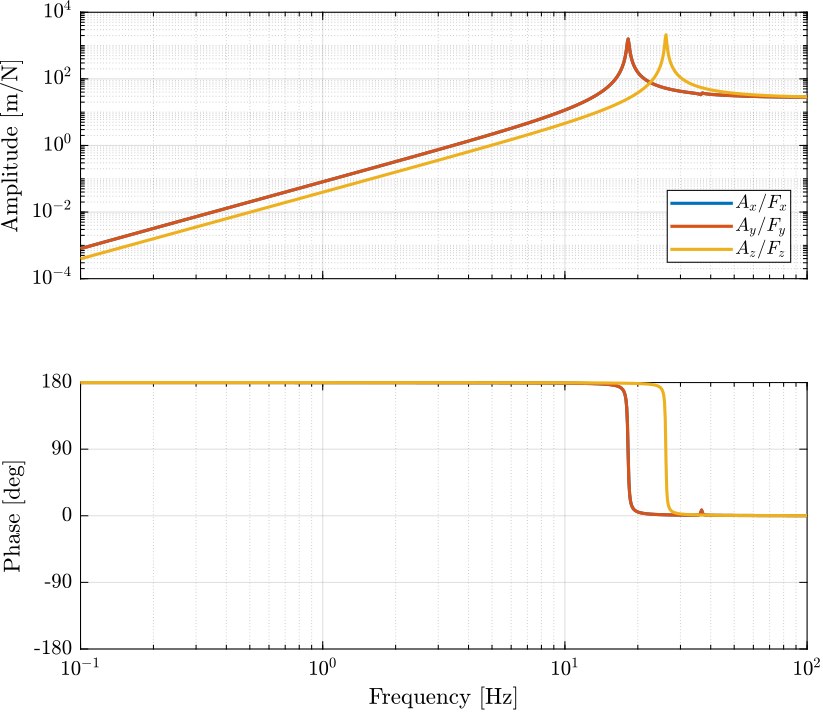
Figure 5: Stewart Platform Plant from forces applied by the legs to the acceleration of the platform

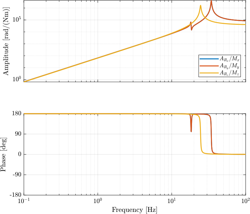
Figure 6: Stewart Platform Plant from torques applied by the legs to the angular acceleration of the platform

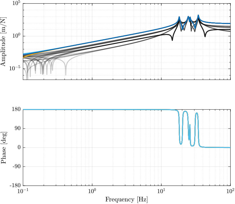
Figure 7: Stewart Platform Plant from forces applied by the legs to displacement of the legs

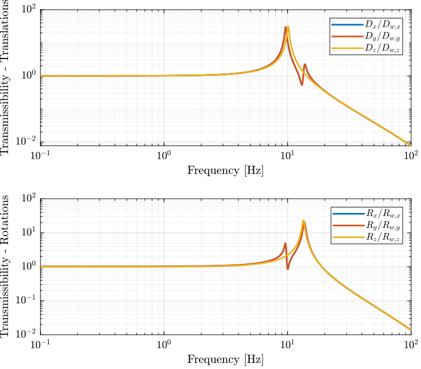
Figure 8: Transmissibility

3.5 Real Approximation of \(G\) at the decoupling frequency

Let’s compute a real approximation of the complex matrix \(H_1\) which corresponds to the the transfer function \(G_c(j\omega_c)\) from forces applied by the actuators to the measured acceleration of the top platform evaluated at the frequency \(\omega_c\).

wc = 2*pi*20; % Decoupling frequency [rad/s]

Gc = G({'Ax', 'Ay', 'Az', 'Arx', 'Ary', 'Arz'}, ...
       {'F1', 'F2', 'F3', 'F4', 'F5', 'F6'}); % Transfer function to find a real approximation

H1 = evalfr(Gc, j*wc);

The real approximation is computed as follows:

D = pinv(real(H1'*H1));
H1 = inv(D*real(H1'*diag(exp(j*angle(diag(H1*D*H1.'))/2))));

3.6 Verification of the decoupling using the “Gershgorin Radii”

First, the Singular Value Decomposition of \(H_1\) is performed: \[ H_1 = U \Sigma V^H \]

[U,S,V] = svd(H1);

Then, the “Gershgorin Radii” is computed for the plant \(G_c(s)\) and the “SVD Decoupled Plant” \(G_d(s)\): \[ G_d(s) = U^T G_c(s) V \]

This is computed over the following frequencies.

freqs = logspace(-2, 2, 1000); % [Hz]

Gershgorin Radii for the coupled plant:

Gr_coupled = zeros(length(freqs), size(Gc,2));

H = abs(squeeze(freqresp(Gc, freqs, 'Hz')));
for out_i = 1:size(Gc,2)
    Gr_coupled(:, out_i) = squeeze((sum(H(out_i,:,:)) - H(out_i,out_i,:))./H(out_i, out_i, :));
end

Gershgorin Radii for the decoupled plant using SVD:

Gd = U'*Gc*V;
Gr_decoupled = zeros(length(freqs), size(Gd,2));

H = abs(squeeze(freqresp(Gd, freqs, 'Hz')));
for out_i = 1:size(Gd,2)
    Gr_decoupled(:, out_i) = squeeze((sum(H(out_i,:,:)) - H(out_i,out_i,:))./H(out_i, out_i, :));
end

Gershgorin Radii for the decoupled plant using the Jacobian:

Gj = Gc*inv(J');
Gr_jacobian = zeros(length(freqs), size(Gj,2));

H = abs(squeeze(freqresp(Gj, freqs, 'Hz')));

for out_i = 1:size(Gj,2)
    Gr_jacobian(:, out_i) = squeeze((sum(H(out_i,:,:)) - H(out_i,out_i,:))./H(out_i, out_i, :));
end

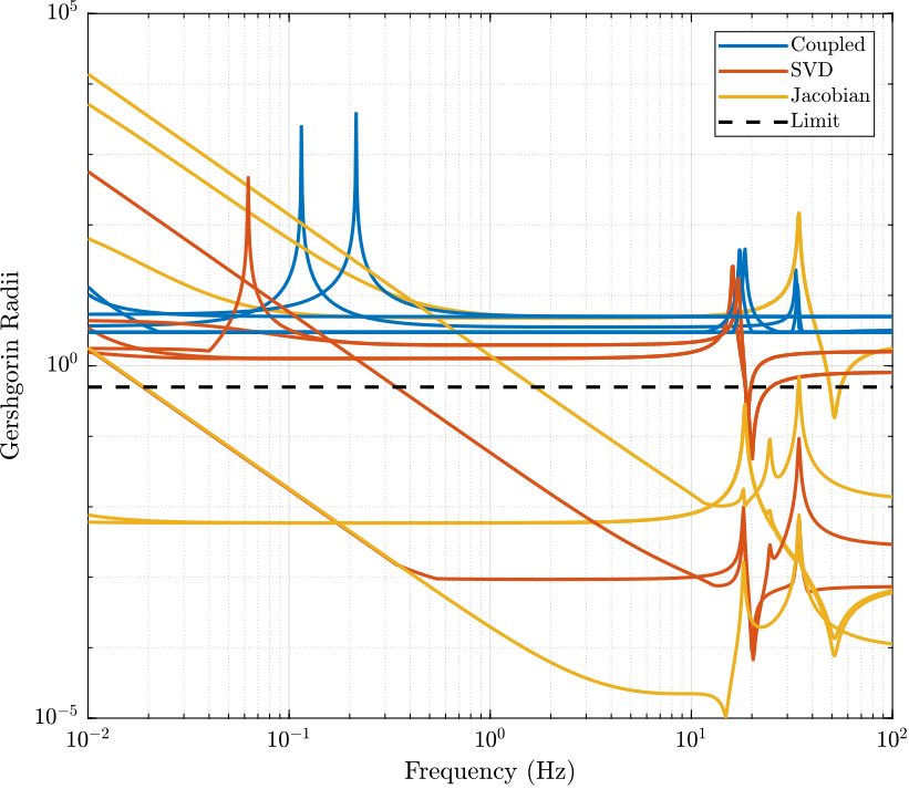
Figure 9: Gershgorin Radii of the Coupled and Decoupled plants

3.7 Decoupled Plant

Let’s see the bode plot of the decoupled plant \(G_d(s)\). \[ G_d(s) = U^T G_c(s) V \]

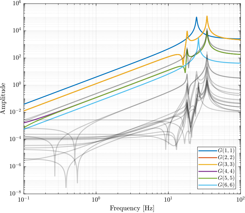
Figure 10: Decoupled Plant using SVD

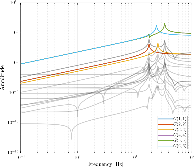
Figure 11: Decoupled Plant using the Jacobian

3.8 Diagonal Controller

The controller \(K\) is a diagonal controller consisting a low pass filters with a crossover frequency \(\omega_c\) and a DC gain \(C_g\).

wc = 2*pi*0.1; % Crossover Frequency [rad/s]
C_g = 50; % DC Gain

K = eye(6)*C_g/(s+wc);

3.9 Centralized Control

The control diagram for the centralized control is shown below.

The controller \(K_c\) is “working” in an cartesian frame. The Jacobian is used to convert forces in the cartesian frame to forces applied by the actuators.

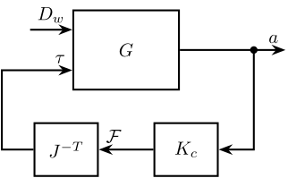
G_cen = feedback(G, inv(J')*K, [7:12], [1:6]);

3.10 SVD Control

The SVD control architecture is shown below. The matrices \(U\) and \(V\) are used to decoupled the plant \(G\).

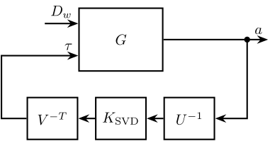
SVD Control

G_svd = feedback(G, pinv(V')*K*pinv(U), [7:12], [1:6]);

3.11 Results

Let’s first verify the stability of the closed-loop systems:

isstable(G_cen)

ans =
  logical
   1

isstable(G_svd)

ans =
  logical
   0

The obtained transmissibility in Open-loop, for the centralized control as well as for the SVD control are shown in Figure 14.

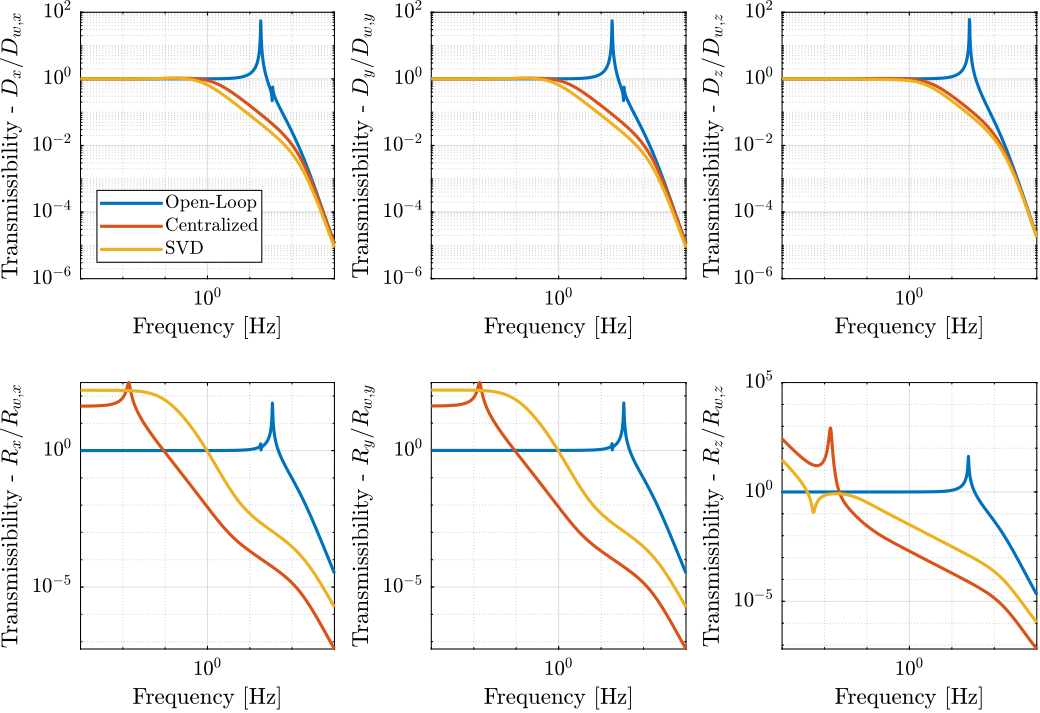
Figure 14: Obtained Transmissibility

4 Stewart Platform - Analytical Model

4.1 Characteristics

L  = 0.055; % Leg length [m]
Zc = 0;     % ?
m  = 0.2;   % Top platform mass [m]
k  = 1e3;   % Total vertical stiffness [N/m]
c  = 2*0.1*sqrt(k*m); % Damping ? [N/(m/s)]

Rx = 0.04; % ?
Rz = 0.04; % ?
Ix = m*Rx^2; % ?
Iy = m*Rx^2; % ?
Iz = m*Rz^2; % ?

4.2 Mass Matrix

M = m*[1   0 0  0         Zc        0;
       0   1 0 -Zc        0         0;
       0   0 1  0         0         0;
       0 -Zc 0  Rx^2+Zc^2 0         0;
       Zc  0 0  0         Rx^2+Zc^2 0;
       0   0 0  0         0         Rz^2];

4.3 Jacobian Matrix

Bj=1/sqrt(6)*[ 1             1          -2          1         1        -2;
               sqrt(3)      -sqrt(3)     0          sqrt(3)  -sqrt(3)   0;
               sqrt(2)       sqrt(2)     sqrt(2)    sqrt(2)   sqrt(2)   sqrt(2);
               0             0           L          L        -L         -L;
               -L*2/sqrt(3) -L*2/sqrt(3) L/sqrt(3)  L/sqrt(3) L/sqrt(3)  L/sqrt(3);
               L*sqrt(2)    -L*sqrt(2)   L*sqrt(2) -L*sqrt(2) L*sqrt(2) -L*sqrt(2)];

4.4 Stifnness and Damping matrices

kv = k/3;     % Vertical Stiffness of the springs [N/m]
kh = 0.5*k/3; % Horizontal Stiffness of the springs [N/m]

K = diag([3*kh, 3*kh, 3*kv, 3*kv*Rx^2/2, 3*kv*Rx^2/2, 3*kh*Rx^2]); % Stiffness Matrix
C = c*K/100000; % Damping Matrix

4.5 State Space System

A  = [ zeros(6) eye(6); ...
      -M\K     -M\C];
Bw = [zeros(6); -eye(6)];
Bu = [zeros(6); M\Bj];

Co = [-M\K -M\C];

D  = [zeros(6) M\Bj];

ST = ss(A,[Bw Bu],Co,D);

OUT 1-6: 6 dof
IN 1-6 : ground displacement in the directions of the legs
IN 7-12: forces in the actuators.

ST.StateName = {'x';'y';'z';'theta_x';'theta_y';'theta_z';...
                'dx';'dy';'dz';'dtheta_x';'dtheta_y';'dtheta_z'};

ST.InputName = {'w1';'w2';'w3';'w4';'w5';'w6';...
                'u1';'u2';'u3';'u4';'u5';'u6'};

ST.OutputName = {'ax';'ay';'az';'atheta_x';'atheta_y';'atheta_z'};

4.6 Transmissibility

TR=ST*[eye(6); zeros(6)];

figure
subplot(231)
bodemag(TR(1,1));
subplot(232)
bodemag(TR(2,2));
subplot(233)
bodemag(TR(3,3));
subplot(234)
bodemag(TR(4,4));
subplot(235)
bodemag(TR(5,5));
subplot(236)
bodemag(TR(6,6));

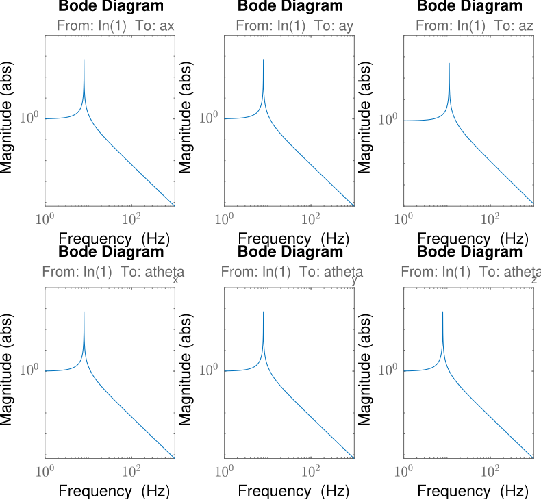
Figure 15: Transmissibility

4.7 Real approximation of \(G(j\omega)\) at decoupling frequency

sys1 = ST*[zeros(6); eye(6)]; % take only the forces inputs

dec_fr = 20;
H1 = evalfr(sys1,j*2*pi*dec_fr);
H2 = H1;
D = pinv(real(H2'*H2));
H1 = inv(D*real(H2'*diag(exp(j*angle(diag(H2*D*H2.'))/2)))) ;
[U,S,V] = svd(H1);

wf = logspace(-1,2,1000);
for i  = 1:length(wf)
    H = abs(evalfr(sys1,j*2*pi*wf(i)));
    H_dec = abs(evalfr(U'*sys1*V,j*2*pi*wf(i)));
    for j = 1:size(H,2)
        g_r1(i,j) =  (sum(H(j,:))-H(j,j))/H(j,j);
        g_r2(i,j) =  (sum(H_dec(j,:))-H_dec(j,j))/H_dec(j,j);
        %     keyboard
    end
    g_lim(i) = 0.5;
end

4.8 Coupled and Decoupled Plant “Gershgorin Radii”

figure;
title('Coupled plant')
loglog(wf,g_r1(:,1),wf,g_r1(:,2),wf,g_r1(:,3),wf,g_r1(:,4),wf,g_r1(:,5),wf,g_r1(:,6),wf,g_lim,'--');
legend('$a_x$','$a_y$','$a_z$','$\theta_x$','$\theta_y$','$\theta_z$','Limit');
xlabel('Frequency (Hz)'); ylabel('Gershgorin Radii')

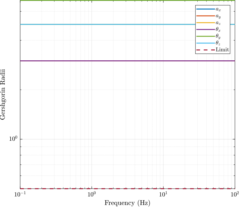
Figure 16: Gershorin Raddi for the coupled plant

figure;
title('Decoupled plant (10 Hz)')
loglog(wf,g_r2(:,1),wf,g_r2(:,2),wf,g_r2(:,3),wf,g_r2(:,4),wf,g_r2(:,5),wf,g_r2(:,6),wf,g_lim,'--');
legend('$S_1$','$S_2$','$S_3$','$S_4$','$S_5$','$S_6$','Limit');
xlabel('Frequency (Hz)'); ylabel('Gershgorin Radii')

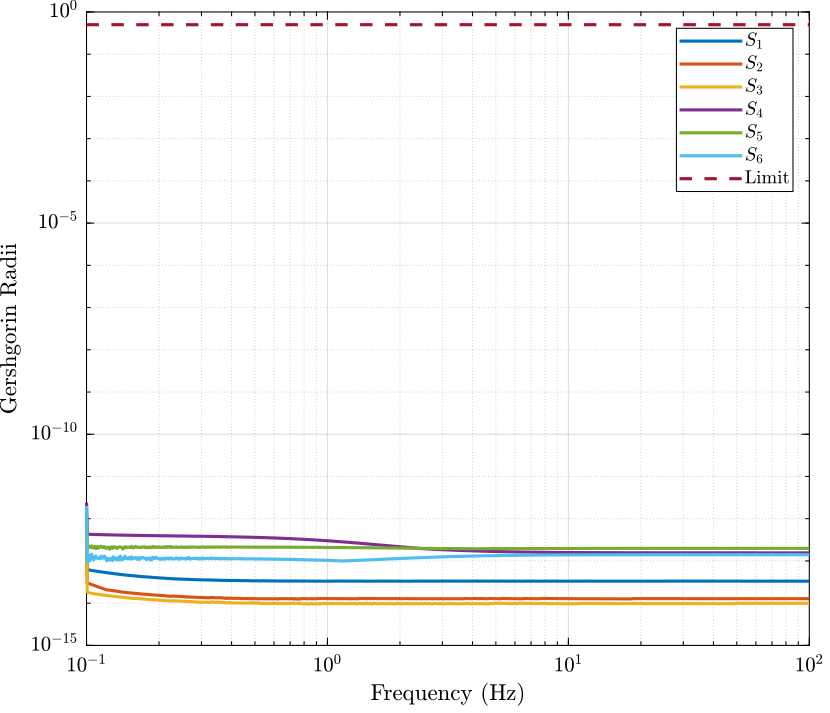
Figure 17: Gershorin Raddi for the decoupled plant

4.9 Decoupled Plant

figure;
bodemag(U'*sys1*V,opts)

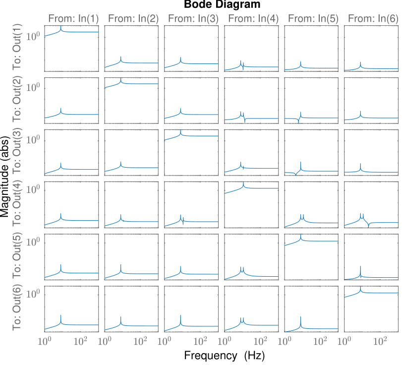
Figure 18: Decoupled Plant

4.10 Controller

fc = 2*pi*0.1; % Crossover Frequency [rad/s]
c_gain = 50; %

cont = eye(6)*c_gain/(s+fc);

4.11 Closed Loop System

FEEDIN  = [7:12]; % Input of controller
FEEDOUT = [1:6]; % Output of controller

Centralized Control

STcen = feedback(ST, inv(Bj)*cont, FEEDIN, FEEDOUT);
TRcen = STcen*[eye(6); zeros(6)];

SVD Control

STsvd = feedback(ST, pinv(V')*cont*pinv(U), FEEDIN, FEEDOUT);
TRsvd = STsvd*[eye(6); zeros(6)];

4.12 Results

figure
subplot(231)
bodemag(TR(1,1),TRcen(1,1),TRsvd(1,1),opts)
legend('OL','Centralized','SVD')
subplot(232)
bodemag(TR(2,2),TRcen(2,2),TRsvd(2,2),opts)
legend('OL','Centralized','SVD')
subplot(233)
bodemag(TR(3,3),TRcen(3,3),TRsvd(3,3),opts)
legend('OL','Centralized','SVD')
subplot(234)
bodemag(TR(4,4),TRcen(4,4),TRsvd(4,4),opts)
legend('OL','Centralized','SVD')
subplot(235)
bodemag(TR(5,5),TRcen(5,5),TRsvd(5,5),opts)
legend('OL','Centralized','SVD')
subplot(236)
bodemag(TR(6,6),TRcen(6,6),TRsvd(6,6),opts)
legend('OL','Centralized','SVD')

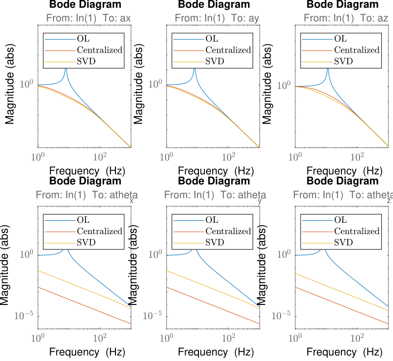
Figure 19: Comparison of the obtained transmissibility for the centralized control and the SVD control

SVD Control

Table of Contents

1 Gravimeter - Simscape Model

1.1 Introduction

1.2 Simscape Model - Parameters

1.3 System Identification - Without Gravity

1.4 System Identification - With Gravity

1.5 Analytical Model

1.5.1 Parameters

1.5.2 Generation of the State Space Model

1.5.3 Comparison with the Simscape Model

1.5.4 Analysis

1.5.5 Control Section

1.5.6 Greshgorin radius

1.5.7 Injecting ground motion in the system to have the output

2 Gravimeter - Functions

2.1 align

2.2 pzmap_testCL

3 Stewart Platform - Simscape Model

3.1 Jacobian

3.2 Simscape Model

3.3 Identification of the plant

3.4 Obtained Dynamics

3.5 Real Approximation of \(G\) at the decoupling frequency

3.6 Verification of the decoupling using the “Gershgorin Radii”

3.7 Decoupled Plant

3.8 Diagonal Controller

3.9 Centralized Control

3.10 SVD Control

3.11 Results

4 Stewart Platform - Analytical Model

4.1 Characteristics

4.2 Mass Matrix

4.3 Jacobian Matrix

4.4 Stifnness and Damping matrices

4.5 State Space System

4.6 Transmissibility

4.7 Real approximation of \(G(j\omega)\) at decoupling frequency

4.8 Coupled and Decoupled Plant “Gershgorin Radii”

4.9 Decoupled Plant

4.10 Controller

4.11 Closed Loop System

4.12 Results

2.1 `align`

2.2 `pzmap_testCL`