Nano-Hexapod

1. Nano-Hexapod
2. Active Damping using Integral Force Feedback
3. Active Damping using Direct Velocity Feedback - Encoders on the struts
4. Active Damping using Direct Velocity Feedback - Encoders on the plates
5. Function - Initialize Nano Hexapod

This report is also available as a pdf.

In this document, a Simscape model of the nano-hexapod is developed and studied.

It is structured as follows:

Section 1: the simscape model of the nano-hexapod is presented. Few of its elements can be configured as wanted. The effect of the configuration on the obtained dynamics is studied.
Section 2: Direct Velocity Feedback is applied and the obtained damping is derived.
Section 3: the encoders are fixed to the struts, and Integral Force Feedback is applied. The obtained damping is computed.
Section 4: the same is done when the encoders are fixed on the plates

1 Nano-Hexapod

1.1 Nano Hexapod - Configuration

The nano-hexapod can be initialized and configured using the initializeNanoHexapodFinal function (link).

The following code would produce the model shown in Figure 1.

n_hexapod = initializeNanoHexapodFinal('flex_bot_type', '4dof', ...
                                       'flex_top_type', '3dof', ...
                                       'motion_sensor_type', 'struts', ...
                                       'actuator_type', '2dof', ...
                                       'MO_B', 150e-3);

Figure 1: 3D view of the Sismcape model for the Nano-Hexapod

Several elements on the nano-hexapod can be configured:

The flexible joints (Section 1.1.1)
The amplified piezoelectric actuators (Section 1.1.2)
The encoders (Section 1.1.3)
The Jacobian matrices (Section 1.1.4)

1.1.1 Flexible Joints

The model of the flexible joint is composed of 3 solid bodies as shown in Figure 2 which are connected by joints representing the flexibility of the joint.

We can represent:

the bending flexibility \(k_{R_x}\), \(k_{R_y}\)
the torsional flexibility \(k_{R_z}\)
the axial flexibility \(k_z\)

The configurations and the represented flexibilities are summarized in Table 1.

Table 1: Flexible joint’s configuration and associated represented flexibility
`flex_type`	Bending	Torsional	Axial
`2dof`	x
`3dof`	x	x
`4dof`	x	x	x

Of course, adding more DoF for the flexible joint will induce an addition of many states for the nano-hexapod simscape model.

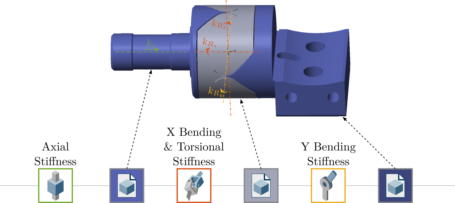
Figure 2: 3D view of the Sismcape model for the Flexible joint (4DoF configuration)

1.1.2 Amplified Piezoelectric Actuators

The nano-hexapod’s struts are containing one amplified piezoelectric actuator (APA300ML from Cedrat Technologies).

The APA can be modeled in different ways which can be configured with the actuator_type argument.

The simplest model is a 2-DoF system shown in Figure 3.

Figure 3: Schematic of the 2DoF model for the Amplified Piezoelectric Actuator

Then, a more complex model based on a Finite Element Model can be used.

1.1.3 Encoders

The encoders can be either fixed directly on the struts (Figure 4) or on the two plates (Figure 5).

This can be configured with the motion_sensor_type parameters which can be equal to 'struts' or 'plates'.

Figure 4: 3D view of the Encoders fixed on the struts

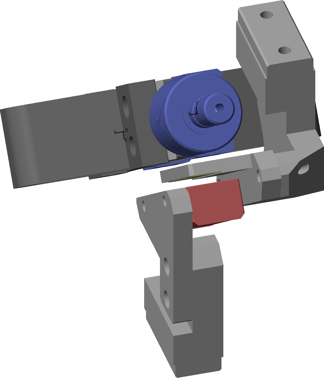
Figure 5: 3D view of the Encoders fixed on the plates

A complete view of the nano-hexapod with encoders fixed to the struts is shown in Figure 1 while it is shown in Figure 6 when the encoders are fixed to the plates.

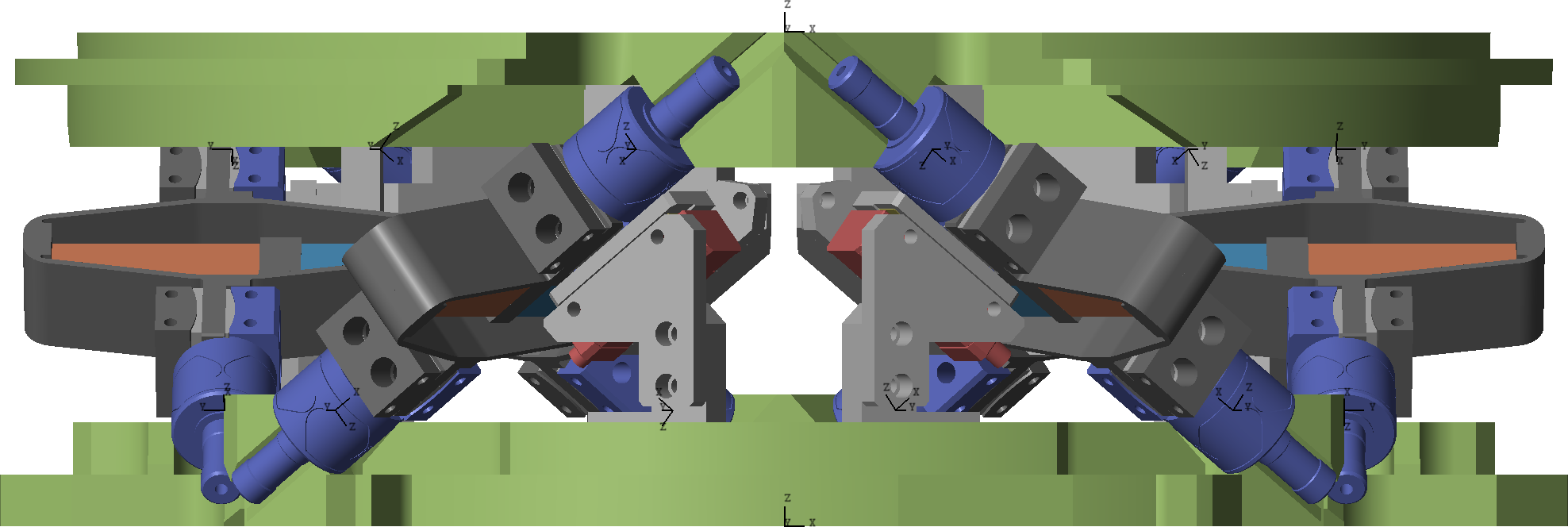
Figure 6: Nano-Hexapod with encoders fixed to the plates

The encoder model is schematically represented in Figure 7:

a frame {B}, fixed to the ruler is positioned on its top surface
a frame {F}, rigidly fixed to the encoder is initially positioned such that its origin is aligned with the x axis of frame {B}

The output measurement is then the x displacement of the origin of the frame {F} expressed in frame {B}.

Figure 7: Schematic of the encoder model

If the encoder is experiencing some tilt, it is then “converted” into a measured displacement as shown in Figure 8.

Figure 8: Schematic of the encoder model

1.1.4 Jacobians

While the Jacobian configuration will not change the physical system, it is still quite an important part of the model.

This configuration consists on defining the location of the frame {B} in which the Jacobian will be computed. This Jacobian is then used to transform the actuator forces to forces/torques applied on the payload and expressed in frame {B}. Same thing can be done for the measured encoder displacements.

1.2 Effect of encoders on the decentralized plant

We here wish to compare the plant from actuators to the encoders when the encoders are either fixed on the struts or on the plates.

We initialize the identification parameters.

%% Options for Linearized
options = linearizeOptions;
options.SampleTime = 0;

%% Name of the Simulink File
mdl = 'nano_hexapod';

%% Input/Output definition
clear io; io_i = 1;
io(io_i) = linio([mdl, '/F'],  1, 'openinput');  io_i = io_i + 1; % Actuator Inputs
io(io_i) = linio([mdl, '/D'],  1, 'openoutput'); io_i = io_i + 1; % Relative Motion Outputs

Identify the plant when the encoders are on the struts:

n_hexapod = initializeNanoHexapodFinal('flex_bot_type', '4dof', ...
                                       'flex_top_type', '3dof', ...
                                       'motion_sensor_type', 'struts', ...
                                       'actuator_type', '2dof');

Gs = linearize(mdl, io, 0.0, options);
Gs.InputName  = {'F1', 'F2', 'F3', 'F4', 'F5', 'F6'};
Gs.OutputName = {'D1', 'D2', 'D3', 'D4', 'D5', 'D6'};

And identify the plant when the encoders are fixed on the plates:

n_hexapod = initializeNanoHexapodFinal('flex_bot_type', '4dof', ...
                                       'flex_top_type', '3dof', ...
                                       'motion_sensor_type', 'plates', ...
                                       'actuator_type', '2dof');

Gp = linearize(mdl, io, 0.0, options);
Gp.InputName  = {'F1', 'F2', 'F3', 'F4', 'F5', 'F6'};
Gp.OutputName = {'D1', 'D2', 'D3', 'D4', 'D5', 'D6'};

The obtained plants are compared in Figure 9.

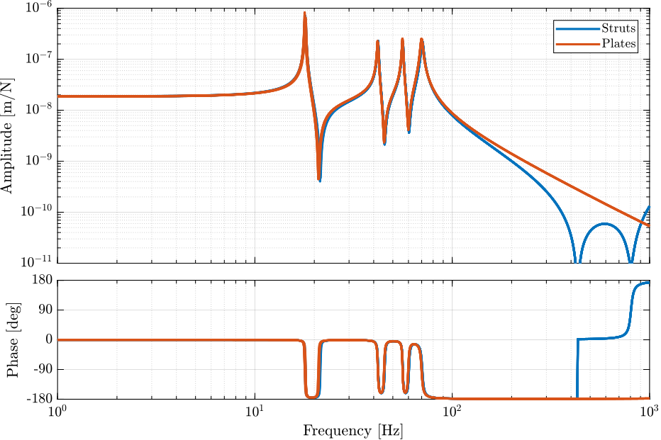
Figure 9: Comparison of the plants from actuator to associated encoder when the encoders are either fixed to the struts or to the plates

Why do we have zeros at 400Hz and 800Hz when the encoders are fixed on the struts?

1.3 Effect of APA flexibility

First identify the plant for APA represented by 2DoF system:

n_hexapod = initializeNanoHexapodFinal('flex_bot_type', '4dof', ...
                                       'flex_top_type', '3dof', ...
                                       'motion_sensor_type', 'struts', ...
                                       'actuator_type', '2dof', ...
                                       'actuator_Ga', 2);

Gs = linearize(mdl, io, 0.0, options);
Gs.InputName  = {'F1', 'F2', 'F3', 'F4', 'F5', 'F6'};
Gs.OutputName = {'D1', 'D2', 'D3', 'D4', 'D5', 'D6'};

First identify the plant for APA represented by a flexible element:

n_hexapod = initializeNanoHexapodFinal('flex_bot_type', '4dof', ...
                                       'flex_top_type', '3dof', ...
                                       'motion_sensor_type', 'struts', ...
                                       'actuator_type', 'flexible');

Gf = linearize(mdl, io, 0.0, options);
Gf.InputName  = {'F1', 'F2', 'F3', 'F4', 'F5', 'F6'};
Gf.OutputName = {'D1', 'D2', 'D3', 'D4', 'D5', 'D6'};

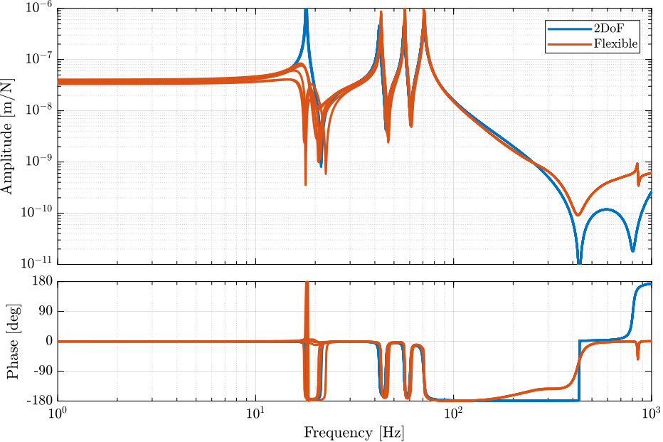
Figure 10: Comparison of the plants from actuator to associated strut encoder when the APA are modelled with a 2DoF system of with a flexible one

The first resonance is strange when using the flexible APA model (Figure 10). Moreover the system is unstable. Otherwise, the 2DoF model matches quite well the flexible model considering its simplicity.

1.4 Nano Hexapod - Number of DoF

In this section, we wish to see how the configuration of each element changes the number of the states of the obtained system.

The most minimalist model is the following:

n_hexapod = initializeNanoHexapodFinal('flex_bot_type', '3dof', ...
                                       'flex_top_type', '2dof', ...
                                       'motion_sensor_type', 'struts', ...
                                       'actuator_type', '2dof');
G = linearize(mdl, io, 0.0, options);

There are 24 states.

These states are summarized on table 2.

Table 2: Number of states for the minimalist model
Element	States
Struts	2*6
Top Plate	12
Total:	24

If we add axial stiffness on the top joints, we should add 2 states for each struts.

n_hexapod = initializeNanoHexapodFinal('flex_bot_type', '4dof', ...
                                       'flex_top_type', '2dof', ...
                                       'motion_sensor_type', 'struts', ...
                                       'actuator_type', '2dof');
G = linearize(mdl, io, 0.0, options);

There are 36 states.

If we add torsional stiffness on the bottom joints, we should again add 2 states for each struts.

n_hexapod = initializeNanoHexapodFinal('flex_bot_type', '4dof', ...
                                       'flex_top_type', '3dof', ...
                                       'motion_sensor_type', 'struts', ...
                                       'actuator_type', '2dof');
G = linearize(mdl, io, 0.0, options);

There are 48 states.

Finally, if we add axial stiffness on the bottom joint, we should add 2 states for each struts.

n_hexapod = initializeNanoHexapodFinal('flex_bot_type', '4dof', ...
                                       'flex_top_type', '4dof', ...
                                       'motion_sensor_type', 'struts', ...
                                       'actuator_type', '2dof');
G = linearize(mdl, io, 0.0, options);

There are 60 states.

Obtained number of states is very comprehensible. Depending on the physical effects we want to model, we therefore know how many states are added when configuring the model.

1.5 Direct Velocity Feedback Plant

The transfer function from actuator forces \(\tau_i\) to the encoder measurements \(\mathcal{L}_i\) is now identified both when the encoders are fixed to the struts.

%% Options for Linearized
options = linearizeOptions;
options.SampleTime = 0;

%% Name of the Simulink File
mdl = 'nano_hexapod';

%% Input/Output definition
clear io; io_i = 1;
io(io_i) = linio([mdl, '/F'], 1, 'openinput');  io_i = io_i + 1; % Actuator Inputs [N]
io(io_i) = linio([mdl, '/D'], 1, 'openoutput'); io_i = io_i + 1; % Relative displacements [m]

n_hexapod = initializeNanoHexapodFinal('flex_bot_type', '4dof', ...
                                       'flex_top_type', '3dof', ...
                                       'motion_sensor_type', 'struts', ...
                                       'actuator_type', '2dof');

Gdvf = linearize(mdl, io, 0.0, options);

The DC gain from actuator to relative motion sensor should be equal to (for the 2dof APA): \[ \frac{1}{k + k_a + kk_a/k_e} \]

Which is equal to:

DCgain = 1.87e-08 [m/N]

Let’s verify that by looking at the DC gain of the \(6 \times 6\) DVF plant in Table 3.

Table 3: DC gain of the DVF plant
1.8617e-08	-1.0408e-10	1.3034e-10	3.2559e-11	-1.1188e-10	9.0385e-11
-5.1839e-11	1.8593e-08	-4.4868e-11	8.016e-11	4.3558e-11	-1.1164e-10
5.1963e-12	-6.9001e-12	1.8564e-08	3.0844e-11	4.0097e-11	-3.4387e-11
1.9359e-11	1.7432e-10	-5.0928e-11	1.855e-08	1.6406e-10	4.5757e-12
-2.1185e-11	2.1724e-10	1.5333e-12	-8.802e-11	1.8803e-08	-4.6946e-11
-1.1728e-11	-5.7682e-11	1.6213e-10	2.1934e-12	-1.6237e-10	1.8715e-08

And the bode plot of the DVF plant is shown in Figure 11.

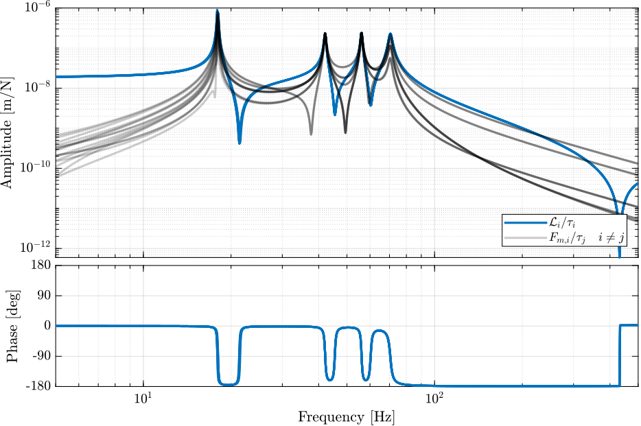
Figure 11: Bode plot of the transfer functions from actuator forces \(\tau_i\) to relative motion sensors attached to the struts \(\mathcal{L}_i\). Diagonal terms are shown in blue, and off-diagonal terms in black.

1.6 Integral Force Feedback Plant

The transfer function from actuators to force sensors is identified.

%% Options for Linearized
options = linearizeOptions;
options.SampleTime = 0;

%% Name of the Simulink File
mdl = 'nano_hexapod';

%% Input/Output definition
clear io; io_i = 1;
io(io_i) = linio([mdl, '/F'],  1, 'openinput');   io_i = io_i + 1; % Actuator Inputs
io(io_i) = linio([mdl, '/Fm'],  1, 'openoutput'); io_i = io_i + 1; % Force Sensors

n_hexapod = initializeNanoHexapodFinal('flex_bot_type', '4dof', ...
                                       'flex_top_type', '3dof', ...
                                       'motion_sensor_type', 'struts', ...
                                       'actuator_type', '2dof');

Giff = linearize(mdl, io, 0.0, options);

This is corresponding to the dynamics for the Integral Force Feedback (IFF) control strategy.

The bode plot is shown in Figure 12.

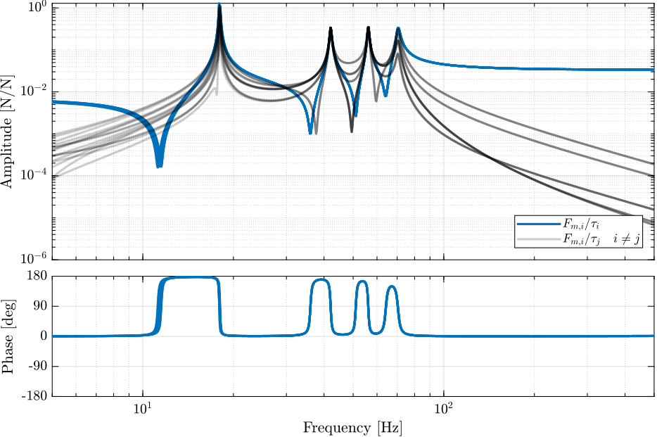
Figure 12: Bode plot of the transfer functions from actuator forces \(\tau_i\) to force sensors \(F_{m,i}\). Diagonal terms are shown in blue, and off-diagonal terms in black.

1.7 Decentralized Plant - Cartesian coordinates

Consider the plant shown in Figure 13 with:

\(\tau\) the 6 input forces (APA)
\(d\mathcal{L}\) the relative motion sensor outputs (encoders)
\(\mathcal{X}\) the motion of the top platform measured with “perfect” 6-dof sensor
\(J_a\) and \(J_s\) the Jacobians for the actuators and sensors

Figure 13: Plant in the cartesian Frame

1.7.1 Verification of the Sensor Jacobian

The “perfect” sensor output \(\mathcal{X}\) is used to verify that the sensor Jacobian is working correctly both when the encoders are fixed to the struts and to the plates.

Let’s then identify the plant for both configuration, and compare the transfer functions from \(\mathcal{F}\) to \(d\mathcal{X}\) and to \(\mathcal{X}\).

%% Options for Linearized
options = linearizeOptions;
options.SampleTime = 0;

%% Name of the Simulink File
mdl = 'nano_hexapod';

%% Input/Output definition
clear io; io_i = 1;
io(io_i) = linio([mdl, '/F'],  1, 'openinput');  io_i = io_i + 1; % Actuator Inputs
io(io_i) = linio([mdl, '/D'],  1, 'openoutput'); io_i = io_i + 1; % Relative Motion Outputs
io(io_i) = linio([mdl, '/X'],  1, 'openoutput'); io_i = io_i + 1; % Relative Motion Outputs

Start when the encoders are fixed on the struts.

n_hexapod = initializeNanoHexapodFinal('flex_bot_type', '4dof', ...
                                       'flex_top_type', '3dof', ...
                                       'motion_sensor_type', 'struts', ...
                                       'actuator_type', '2dof', ...
                                       'MO_B', 150e-3);
Gs = linearize(mdl, io, 0.0, options);
Gs.InputName  = {'F1', 'F2', 'F3', 'F4', 'F5', 'F6'};
Gs.OutputName = {'D1', 'D2', 'D3', 'D4', 'D5', 'D6', ...
                 'Dx', 'Dy', 'Dz', 'Rx', 'Ry', 'Rz'};

% Cartesian plant using the Jacobians
Gsc = inv(n_hexapod.geometry.Js)*Gs({'D1', 'D2', 'D3', 'D4', 'D5', 'D6'}, {'F1', 'F2', 'F3', 'F4', 'F5', 'F6'})*inv(n_hexapod.geometry.J)';
% Cartesian plant using the perfect sensor
Gsp = -Gs({'Dx', 'Dy', 'Dz', 'Rx', 'Ry', 'Rz'}, {'F1', 'F2', 'F3', 'F4', 'F5', 'F6'})*inv(n_hexapod.geometry.J)';

The diagonal elements of the plant are shown in Figure 14.

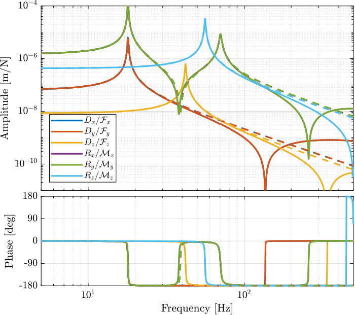
Figure 14: Bode plot of the diagonal elements of the decentralized (cartesian) plant when using the sensor Jacobian (solid) and when using “perfect” 6dof sensor (dashed). The encoders are fixed on the struts.

The same if performed when the encoders are fixed to the plates.

n_hexapod = initializeNanoHexapodFinal('flex_bot_type', '4dof', ...
                                       'flex_top_type', '3dof', ...
                                       'motion_sensor_type', 'plates', ...
                                       'actuator_type', '2dof', ...
                                       'MO_B', 150e-3);
Gp = linearize(mdl, io, 0.0, options);
Gp.InputName  = {'F1', 'F2', 'F3', 'F4', 'F5', 'F6'};
Gp.OutputName = {'D1', 'D2', 'D3', 'D4', 'D5', 'D6', ...
                 'Dx', 'Dy', 'Dz', 'Rx', 'Ry', 'Rz'};

% Cartesian plant using the Jacobians
Gpc = inv(n_hexapod.geometry.Js)*Gp({'D1', 'D2', 'D3', 'D4', 'D5', 'D6'}, {'F1', 'F2', 'F3', 'F4', 'F5', 'F6'})*inv(n_hexapod.geometry.J)';
% Cartesian plant using the perfect sensor
Gpp = -Gp({'Dx', 'Dy', 'Dz', 'Rx', 'Ry', 'Rz'}, {'F1', 'F2', 'F3', 'F4', 'F5', 'F6'})*inv(n_hexapod.geometry.J)';

The obtained bode plots are shown in Figure 15.

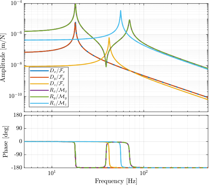
Figure 15: Bode plot of the diagonal elements of the decentralized (cartesian) plant when using the sensor Jacobian (solid) and when using “perfect” 6dof sensor (dashed). The encoders are fixed on the plates.

The Jacobian for the encoders is working properly both when the encoders are fixed to the plates or to the struts.

However, then the encoders are fixed to the struts, there is a mismatch between the estimated motion and the measured motion above 100Hz due to a complex conjugate zero.

1.7.2 Comparison of the decentralized plants

The decentralized plants are now compared whether the encoders are fixed on the struts or on the plates in Figure 16.

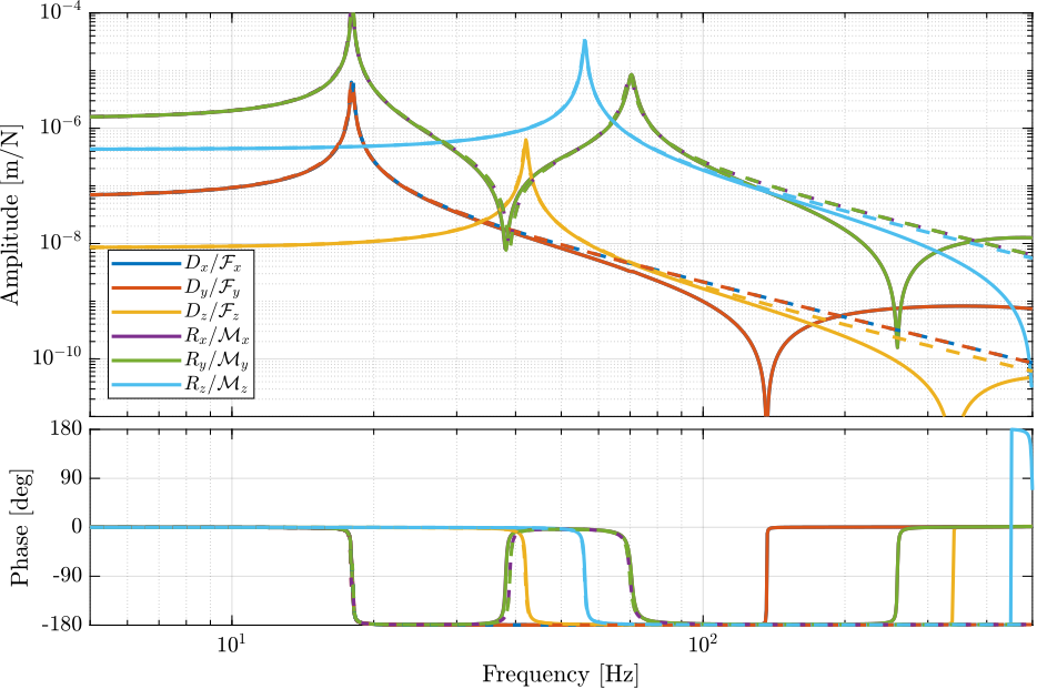
Figure 16: Bode plot of the “cartesian” plant (transfer function from \(\mathcal{F}\) to \(d\mathcal{X}\)) when the encoders are fixed on the struts (solid) and on the plates (dashed)

1.8 Decentralized Plant - Decoupling at the Center of Stiffness

1.8.1 Center of Stiffness

Let’s define some parameters that will be used for the computation of the stiffness matrix:

si = n_hexapod.geometry.si; % Orientation of struts
bi = n_hexapod.geometry.Fb; % Location of bi w.r.t. {F}
ki = ones(1,6); % Normalized strut stiffness

In order to find is the Center of Stiffness (CoK) exists, we have to verify is the following is diagonal:

ki.*si*si'

1.8977	2.4659e-17	5.1838e-19
2.4659e-17	1.8977	-2.3143e-05
5.1838e-19	-2.3143e-05	2.2046

And we can find the location of the CoK with respect to {F}:

OkX = (ki.*cross(bi, si)*si')/(ki.*si*si');
Ok = [OkX(3,2);OkX(1,3);OkX(2,1)]

-1.7444e-18

2.1511e-06

0.052707

The “center of stiffness” is therefore 52.7mm above the bottom platform {F} frame.

Let’s initialize the hexapod with frame {A} and {B} at the CoK:

n_hexapod = initializeNanoHexapodFinal('flex_bot_type', '4dof', ...
                                       'flex_top_type', '3dof', ...
                                       'motion_sensor_type', 'struts', ...
                                       'actuator_type', '2dof', ...
                                       'MO_B', Ok(3)-95e-3);

And the (normalized) stiffness matrix is computed as follows:

n_hexapod.geometry.J'*diag(ki)*n_hexapod.geometry.J

Table 4: Normalized Stiffness Matrix - Center of Stiffness
1.8977	0	0	0	-2.0817e-17	-1.5311e-06
0	1.8977	-2.3143e-05	4.175e-06	0	0
0	-2.3143e-05	2.2046	4.7422e-06	0	0
0	4.175e-06	4.7422e-06	0.012594	2.1684e-19	-8.6736e-19
-1.8521e-17	0	0	0	0.012594	-9.3183e-08
-1.5311e-06	-6.9389e-18	2.7756e-17	-8.6736e-19	-9.3183e-08	0.043362

And we indeed obtain a diagonal stiffness matrix.

1.8.2 Obtained plant

Let’s identify the transfer function from \(\tau\) to \(d\mathcal{L}\) and from \(\tau\) to \(\mathcal{X}\).

%% Options for Linearized
options = linearizeOptions;
options.SampleTime = 0;

%% Name of the Simulink File
mdl = 'nano_hexapod';

%% Input/Output definition
clear io; io_i = 1;
io(io_i) = linio([mdl, '/F'],  1, 'openinput');  io_i = io_i + 1; % Actuator Inputs
io(io_i) = linio([mdl, '/D'],  1, 'openoutput'); io_i = io_i + 1; % Relative Motion Outputs
io(io_i) = linio([mdl, '/X'],  1, 'openoutput'); io_i = io_i + 1; % 6DoF perfect measurement

G = linearize(mdl, io, 0.0, options);
G.InputName  = {'F1', 'F2', 'F3', 'F4', 'F5', 'F6'};
G.OutputName = {'D1', 'D2', 'D3', 'D4', 'D5', 'D6', ...
                'Dx', 'Dy', 'Dz', 'Rx', 'Ry', 'Rz'};

Then use the Jacobian matrices to obtain the “cartesian” centralized plant.

Gc = inv(n_hexapod.geometry.J)*...
     G({'D1', 'D2', 'D3', 'D4', 'D5', 'D6'}, {'F1', 'F2', 'F3', 'F4', 'F5', 'F6'})*...
     inv(n_hexapod.geometry.J');

The DC gain of the obtained plant is shown in Table 5.

Table 5: DC gain of the centralized plant at the center of stiffness
9.8602e-09	7.8692e-11	1.4426e-11	-2.663e-10	2.8e-10	-4.7559e-11
8.457e-11	9.8788e-09	-2.4002e-11	-2.9502e-11	-1.3262e-10	-8.7346e-11
-4.3244e-11	2.4075e-13	8.4775e-09	1.1442e-11	-2.5809e-10	2.8796e-11
-1.8326e-09	-9.318e-10	6.8188e-10	1.4697e-06	5.5936e-09	8.7632e-10
4.6906e-10	1.5911e-09	1.6989e-10	-5.223e-09	1.4729e-06	-2.6059e-10
-6.5754e-11	-3.0408e-12	5.394e-11	-1.0917e-10	6.9479e-10	4.2979e-07

As the rotations and translations have very different gains, we normalize each motion to one.

Gc = diag(1./diag(dcgain(Gc)))*Gc;

The diagonal and off-diagonal elements are shown in Figure 17, and we can see good decoupling at low frequency.

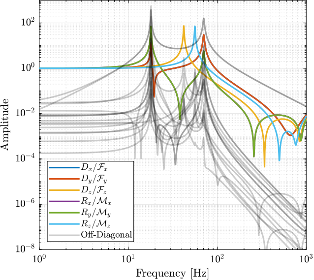
Figure 17: Diagonal and off-diagonal elements of the (normalized) decentralized plant with the Jacobians estimated at the “center of stiffness”

The Jacobian matrices can be used to decoupled the plant at low frequency.

1.9 Stiffness matrix

The stiffness matrix of the nano-hexapod describes its induced static displacement/rotation when a force/torque is applied on its top platform. The location of the applied force/torque and the expressed displacement/rotation can be defined as wanted. Such location (or frame) is then used for the computation of the Jacobian which in turns is used to compute the stiffness matrix.

1.9.1 Compute the theoretical stiffness of the nano-hexapod

Neglecting stiffness of the joints, we have: \[ K = J^t \mathcal{K} J \] where \(\mathcal{K}\) is a diagonal 6x6 matrix with axial stiffness of the struts on the diagonal.

Let’s note the axial stiffness of the APA: \[ k_{\text{APA}} = k + \frac{k_e k_a}{k_e + k_a} \]

Them axial stiffness of the struts \(k_s\): \[ k_s = \frac{k_z k_{\text{APA}}}{k_z + 2 k_{\text{APA}}} \] with \(k_z\) the axial stiffness of the flexible joints.

Let’s initialize the nano-hexapod.

n_hexapod = initializeNanoHexapodFinal('flex_bot_type', '4dof', ...
                                       'flex_top_type', '4dof', ...
                                       'motion_sensor_type', 'struts', ...
                                       'actuator_type', '2dof');

The axial stiffness of the joints and stiffnesses of the 2-DoF actuators are defined below.

k  = n_hexapod.actuator.k(1);
ke = n_hexapod.actuator.ke(1);
ka = n_hexapod.actuator.ka(1);
kz = n_hexapod.flex_top.kz(1); % Joint's axial stiffness [m/N]

The total axial stiffness of the APA is:

kAPA = k + ke*ka/(ke + ka);

kAPA = 1.799e+06 [N/m]

And the total axial stiffness of the struts is:

ks = kz*kAPA/(kz + 2*kAPA);

ks = 1.737e+06 [N/m]

We can see that the axial stiffness of the flexible joint as little impact on the total axial stiffness of the struts.

Let’s now compute the stiffness matrix corresponding to an hexapod with perfect joints and the above computed axial strut stiffness:

Ks = n_hexapod.geometry.J'*(ks*eye(6))*n_hexapod.geometry.J;

And the compliance matrix can be computed as the inverse of the stiffness matrix.

C = inv(Ks);

The obtained compliance matrix is shown in Table 6.

Table 6: Compliance Matrix - Perfect Joints
1.9938e-06	-2.3138e-22	3.3403e-23	1.0202e-21	8.7906e-06	2.9603e-11
-3.1875e-23	1.9938e-06	2.2094e-11	-8.7909e-06	-1.6576e-22	-3.5622e-28
6.6811e-23	2.2094e-11	2.6115e-07	-9.8337e-11	3.4744e-22	7.4663e-28
1.4054e-22	-8.7909e-06	-9.8337e-11	4.5715e-05	7.3086e-22	1.5706e-27
8.7906e-06	-1.0202e-21	1.7371e-22	4.498e-21	4.5714e-05	9.8237e-11
2.9603e-11	-1.9261e-22	-1.7611e-27	8.4925e-22	9.8237e-11	1.3277e-05

1.9.2 Comparison with Simscape Model

Let’s now identify the compliance matrix using Simscape.

%% Options for Linearized
options = linearizeOptions;
options.SampleTime = 0;

%% Name of the Simulink File
mdl = 'nano_hexapod';

%% Input/Output definition
clear io; io_i = 1;
io(io_i) = linio([mdl, '/Fe'],  1, 'openinput');  io_i = io_i + 1; % External forces [N, Nm/rad]
io(io_i) = linio([mdl, '/X'],   1, 'openoutput'); io_i = io_i + 1; % Induced motion [m, rad]

G = linearize(mdl, io, 0.0, options);

The DC gain of the identified plant is therefore the compliance matrix of the nano-hexapod. It takes into account the bending and torsional stiffness of the flexible joints.

The obtained compliance matrix is shown in Table 7.

Table 7: Compliance Matrix - Estimated from Simscape
1.9863e-06	2.4683e-08	2.2859e-09	-6.4768e-08	8.7307e-06	3.2754e-10
-3.693e-09	1.9663e-06	-7.4503e-09	-8.615e-06	-6.7926e-08	-2.0193e-08
-3.5525e-09	-8.8671e-10	2.6042e-07	4.7504e-09	-9.9677e-09	1.7242e-10
2.1133e-08	-8.6554e-06	3.2841e-08	4.4849e-05	3.0873e-07	8.1525e-08
8.7375e-06	9.9165e-08	8.135e-09	-2.5208e-07	4.5331e-05	3.0602e-09
6.1611e-09	6.1733e-09	2.6778e-09	-3.3188e-08	3.3887e-08	1.3212e-05

The bending and torsional stiffness of the flexible joints induces a lot of coupling between forces/torques applied to the to platform to its displacement/rotation. It can be seen by comparison the compliance matrices in Tables 6 and 7.

2 Active Damping using Integral Force Feedback

In this section Integral Force Feedback (IFF) strategy is used to damp the nano-hexapod resonances.

It is structured as follows:

Section 2.1: the IFF plant is identified
Section 2.2: the optimal control gain is identified using the Root Locus plot
Section 2.3: the IFF is applied, and the effect on the damped plant is identified and compared with the un-damped one
Section 2.4: the IFF is applied, and the effect on the compliance is identified

2.1 Plant Identification

The nano-hexapod is initialized as usual.

n_hexapod = initializeNanoHexapodFinal('flex_bot_type', '4dof', ...
                                       'flex_top_type', '4dof', ...
                                       'motion_sensor_type', 'struts', ...
                                       'actuator_type', '2dof');

The transfer function from actuator inputs to force sensors outputs is identified.

%% Options for Linearized
options = linearizeOptions;
options.SampleTime = 0;

%% Name of the Simulink File
mdl = 'nano_hexapod';

%% Input/Output definition
clear io; io_i = 1;
io(io_i) = linio([mdl, '/F'], 1, 'openinput');  io_i = io_i + 1;  % Actuator Inputs
io(io_i) = linio([mdl, '/Fm'], 1, 'openoutput'); io_i = io_i + 1; % Force Sensors

Giff = linearize(mdl, io, 0.0, options);
Giff.InputName  = {'F1',  'F2',  'F3',  'F4',  'F5',  'F6'};
Giff.OutputName = {'Fm1', 'Fm2', 'Fm3', 'Fm4', 'Fm5', 'Fm6'};

Its bode plot is shown in Figure

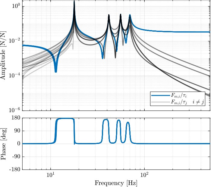
Figure 18: Integral Force Feedback plant

2.2 Root Locus

The controller is a diagonal (i.e. decentralized) controller with simple low pass filters (i.e. pseudo integrators) on the diagonal:

\begin{equation} K_{\text{IFF}} = \frac{g}{s + \omega_c} \bm{I}_{6 \times 6} \end{equation}

The value of \(\omega_c\) has quite a large impact both on the attainable damping and on the compliance degradation at low frequency.

It is here chosen to have quite a large \(\omega_c\) in order to not modify the plant at low frequency.

wc = 2*pi*20;

The obtained Root Locus is shown in Figure 19. The control gain chosen for future plots is shown by the red crosses.

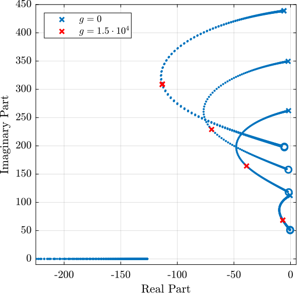
Figure 19: Root locus for the decentralized IFF control strategy

The obtained controller is then:

Kiff = 1.5e4/(s + 2*pi*20)*eye(6); % IFF Controller

The corresponding loop gain of the diagonal terms are shown in Figure 20. It is shown that the loop gain is quite large around resonances (which allows to add lots of damping) and less than one at low frequency thanks to the large value of \(\omega_c\).

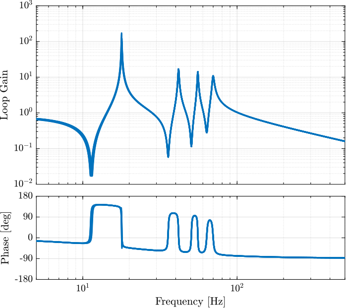
Figure 20: Loop gain of the diagonal terms \(G(i,i) \cdot K_{\text{IFF}}(i,i)\)

2.3 Effect of IFF on the plant

Let’s now see how the IFF control strategy effectively damps the plant and how it affects the transfer functions from the actuator forces to the relative motion sensors (encoders). First identify the plant in open-loop.

n_hexapod = initializeNanoHexapodFinal('flex_bot_type', '4dof', ...
                                       'flex_top_type', '3dof', ...
                                       'motion_sensor_type', 'struts', ...
                                       'actuator_type', '2dof', ...
                                       'controller_type', 'none');

Gol = linearize(mdl, io, 0.0, options);
Gol.InputName  = {'F1', 'F2', 'F3', 'F4', 'F5', 'F6'};
Gol.OutputName = {'D1', 'D2', 'D3', 'D4', 'D5', 'D6'};

And then with the IFF controller.

n_hexapod = initializeNanoHexapodFinal('flex_bot_type', '4dof', ...
                                       'flex_top_type', '3dof', ...
                                       'motion_sensor_type', 'struts', ...
                                       'actuator_type', '2dof', ...
                                       'controller_type', 'iff');

Giff = linearize(mdl, io, 0.0, options);
Giff.InputName  = {'F1', 'F2', 'F3', 'F4', 'F5', 'F6'};
Giff.OutputName = {'D1', 'D2', 'D3', 'D4', 'D5', 'D6'};

The obtained plants are compared in Figure 21.

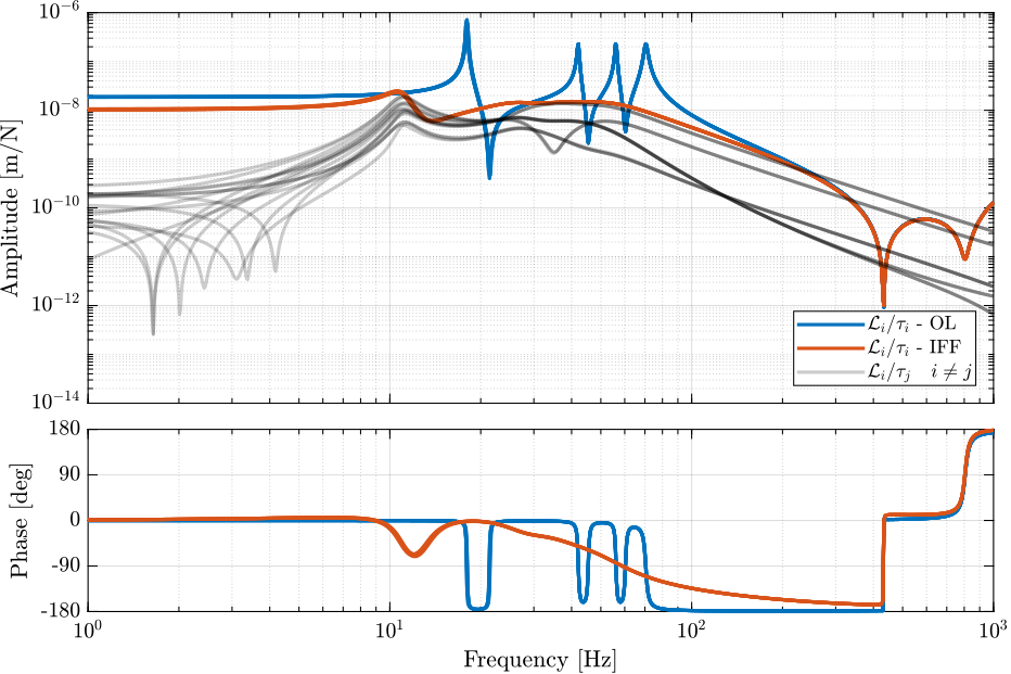
Figure 21: Bode plots of the transfer functions from actuator forces \(\tau_i\) to relative motion sensors \(\mathcal{L}_i\) with and without the IFF controller.

The Integral Force Feedback Strategy is very effective to damp the 6 suspension modes of the nano-hexapod.

2.4 Effect of IFF on the compliance

The IFF strategy has the well known drawback of degrading the compliance (transfer function from external forces/torques applied to the top platform to the motion of the top platform), especially at low frequency where the control gain is large. Let’s quantify that for the nano-hexapod. The obtained compliances are compared in Figure

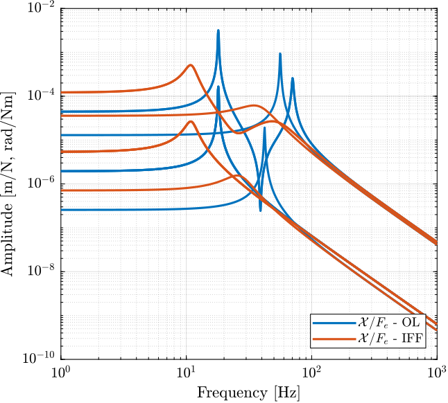
Figure 22: Comparison of the compliances in Open Loop and with Integral Force Feedback controller

The use of IFF induces a degradation of the compliance. This degradation is limited due to the use of a pseudo integrator (instead of a pure integrator). Also, it should not be a major problem for the NASS, as no direct forces should be applied to the top platform.

3 Active Damping using Direct Velocity Feedback - Encoders on the struts

In this section, the Direct Velocity Feedback (DVF) strategy is used to damp the nano-hexapod resonances.

It is structured as follows:

Section 3.1: the DVF plant is identified
Section 3.2: the optimal control gain is identified using the Root Locus plot
Section 3.3: the DVF is applied, and the effect on the damped plant is identified and compared with the un-damped one
Section 3.4: the DVF is applied, and the effect on the compliance is identified

3.1 Plant Identification

The nano-hexapod is initialized as usual.

n_hexapod = initializeNanoHexapodFinal('flex_bot_type', '4dof', ...
                                       'flex_top_type', '4dof', ...
                                       'motion_sensor_type', 'struts', ...
                                       'actuator_type', '2dof');

The transfer function from actuator inputs to force sensors outputs is identified.

%% Options for Linearized
options = linearizeOptions;
options.SampleTime = 0;

%% Name of the Simulink File
mdl = 'nano_hexapod';

%% Input/Output definition
clear io; io_i = 1;
io(io_i) = linio([mdl, '/F'], 1, 'openinput');  io_i = io_i + 1; % Actuator Inputs
io(io_i) = linio([mdl, '/D'], 1, 'openoutput'); io_i = io_i + 1; % Relative Motion Outputs

Gdvf = linearize(mdl, io, 0.0, options);
Gdvf.InputName =  {'F1', 'F2', 'F3', 'F4', 'F5', 'F6'};
Gdvf.OutputName = {'D1', 'D2', 'D3', 'D4', 'D5', 'D6'};

Its bode plot is shown in Figure 23.

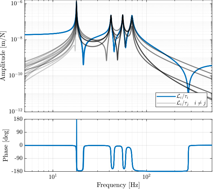
Figure 23: Direct Velocity Feedback plant

3.2 Root Locus

The controller is a diagonal (i.e. decentralized) controller with simple high pass filters (i.e. pseudo derivators) on the diagonal:

\begin{equation} K_{\text{DVF}} = g \frac{s}{s + \omega_d} \bm{I}_{6 \times 6} \end{equation}

The value of \(\omega_d\) sets the frequency above high the derivative action is stopped.

wd = 2*pi*150;

The obtained Root Locus is shown in Figure 24. The control gain chosen for future plots is shown by the red crosses.

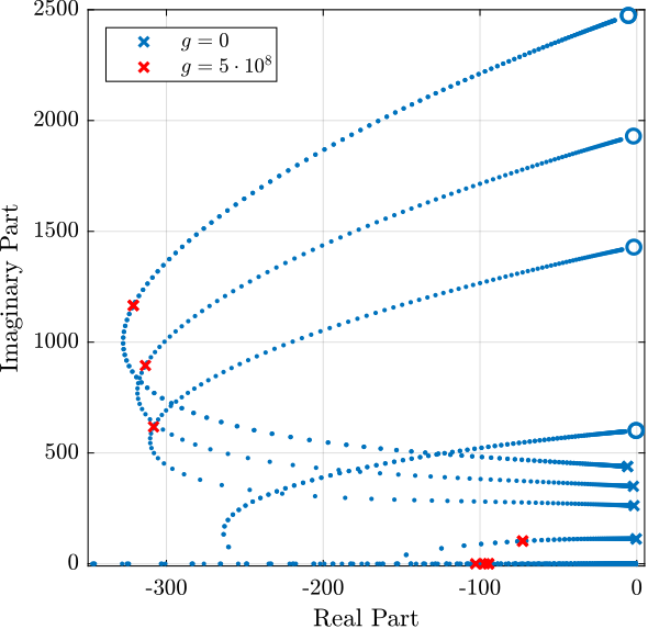
Figure 24: Root locus for the decentralized DVF control strategy

The obtained controller is then:

Kdvf = 5e8*s/(s + wd)*eye(6); % DVF Controller

The corresponding loop gain of the diagonal terms are shown in Figure 25. It is shown that the loop gain is quite large around resonances (which allows to add lots of damping) and less than one at low frequency thanks to the large value of \(\omega_c\).

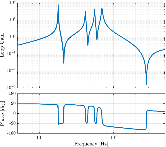
Figure 25: Loop gain of the diagonal terms \(G(i,i) \cdot K_{\text{DVF}}(i,i)\)

3.3 Effect of DVF on the plant

Let’s now see how the DVF control strategy effectively damps the plant and how it affects the transfer functions from the actuator forces to the relative motion sensors (encoders). First identify the plant in open-loop.

n_hexapod = initializeNanoHexapodFinal('flex_bot_type', '4dof', ...
                                       'flex_top_type', '4dof', ...
                                       'motion_sensor_type', 'struts', ...
                                       'actuator_type', '2dof', ...
                                       'controller_type', 'none');

Gol = linearize(mdl, io, 0.0, options);
Gol.InputName  = {'F1', 'F2', 'F3', 'F4', 'F5', 'F6'};
Gol.OutputName = {'D1', 'D2', 'D3', 'D4', 'D5', 'D6'};

And then with the DVF controller.

n_hexapod = initializeNanoHexapodFinal('flex_bot_type', '4dof', ...
                                       'flex_top_type', '4dof', ...
                                       'motion_sensor_type', 'struts', ...
                                       'actuator_type', '2dof', ...
                                       'controller_type', 'dvf');

Gdvf = linearize(mdl, io, 0.0, options);
Gdvf.InputName  = {'F1', 'F2', 'F3', 'F4', 'F5', 'F6'};
Gdvf.OutputName = {'D1', 'D2', 'D3', 'D4', 'D5', 'D6'};

The obtained plants are compared in Figure 26.

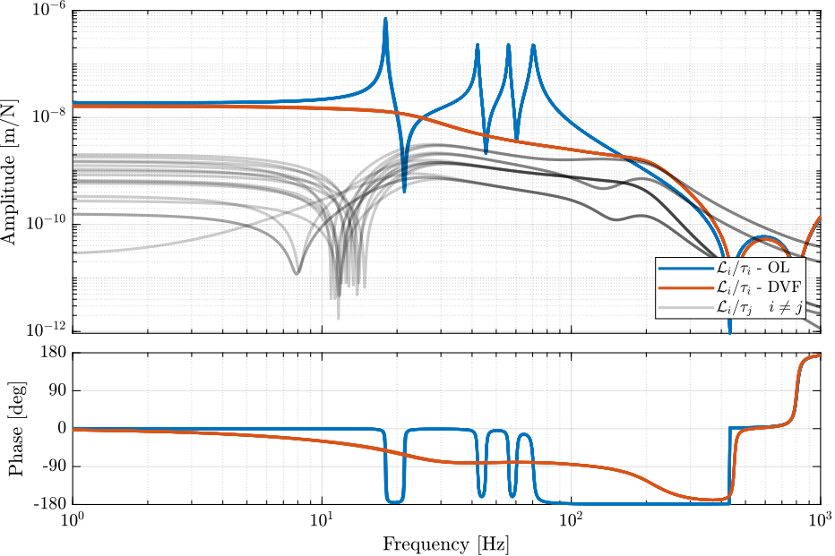
Figure 26: Bode plots of the transfer functions from actuator forces \(\tau_i\) to relative motion sensors \(\mathcal{L}_i\) with and without the DVF controller.

The Direct Velocity Feedback Strategy is very effective to damp the 6 suspension modes of the nano-hexapod.

3.4 Effect of DVF on the compliance

The DVF strategy has the well known drawback of degrading the compliance (transfer function from external forces/torques applied to the top platform to the motion of the top platform), especially at low frequency where the control gain is large. Let’s quantify that for the nano-hexapod. The obtained compliances are compared in Figure 27.

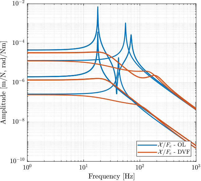
Figure 27: Comparison of the compliances in Open Loop and with Direct Velocity Feedback controller

4 Active Damping using Direct Velocity Feedback - Encoders on the plates

In this section, the Direct Velocity Feedback (DVF) strategy is used to damp the nano-hexapod resonances.

It is structured as follows:

Section 4.1: the DVF plant is identified
Section 4.2: the optimal control gain is identified using the Root Locus plot
Section 4.3: the DVF is applied, and the effect on the damped plant is identified and compared with the un-damped one
Section 4.4: the DVF is applied, and the effect on the compliance is identified

4.1 Plant Identification

The nano-hexapod is initialized as usual.

n_hexapod = initializeNanoHexapodFinal('flex_bot_type', '4dof', ...
                                       'flex_top_type', '4dof', ...
                                       'motion_sensor_type', 'plates', ...
                                       'actuator_type', '2dof');

The transfer function from actuator inputs to force sensors outputs is identified.

%% Options for Linearized
options = linearizeOptions;
options.SampleTime = 0;

%% Name of the Simulink File
mdl = 'nano_hexapod';

%% Input/Output definition
clear io; io_i = 1;
io(io_i) = linio([mdl, '/F'], 1, 'openinput');  io_i = io_i + 1; % Actuator Inputs
io(io_i) = linio([mdl, '/D'], 1, 'openoutput'); io_i = io_i + 1; % Relative Motion Outputs

Gdvf = linearize(mdl, io, 0.0, options);
Gdvf.InputName =  {'F1', 'F2', 'F3', 'F4', 'F5', 'F6'};
Gdvf.OutputName = {'D1', 'D2', 'D3', 'D4', 'D5', 'D6'};

Its bode plot is shown in Figure 28.

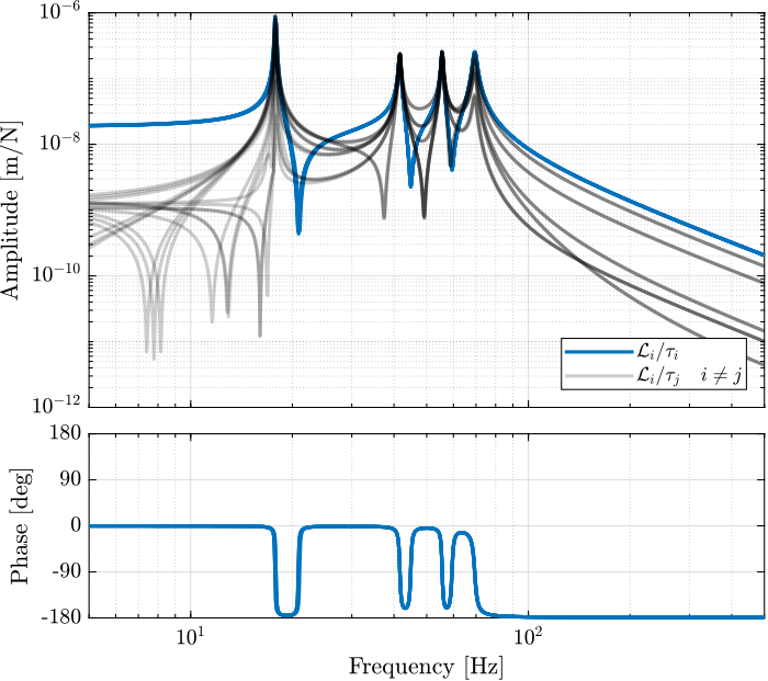
Figure 28: Direct Velocity Feedback plant

4.2 Root Locus

The controller is a diagonal (i.e. decentralized) controller with simple high pass filters (i.e. pseudo derivators) on the diagonal:

\begin{equation} K_{\text{DVF}} = g \frac{s}{s + \omega_d} \bm{I}_{6 \times 6} \end{equation}

The value of \(\omega_d\) sets the frequency above high the derivative action is stopped.

wd = 2*pi*150;

The obtained Root Locus is shown in Figure 29. The control gain chosen for future plots is shown by the red crosses.

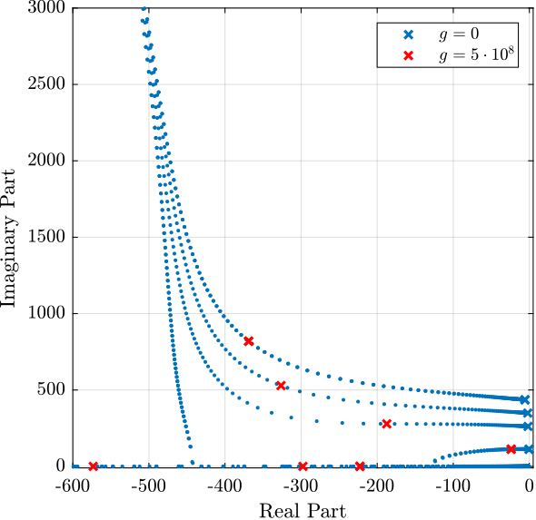
Figure 29: Root locus for the decentralized DVF control strategy

The obtained controller is then:

Kdvf = 2e8*s/(s + wd)*eye(6); % DVF Controller

The corresponding loop gain of the diagonal terms are shown in Figure 30. It is shown that the loop gain is quite large around resonances (which allows to add lots of damping).

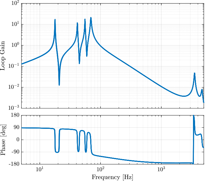
Figure 30: Loop gain of the diagonal terms \(G(i,i) \cdot K_{\text{DVF}}(i,i)\)

4.3 Effect of DVF on the plant

n_hexapod = initializeNanoHexapodFinal('flex_bot_type', '4dof', ...
                                       'flex_top_type', '4dof', ...
                                       'motion_sensor_type', 'plates', ...
                                       'actuator_type', '2dof', ...
                                       'controller_type', 'none');

Gol = linearize(mdl, io, 0.0, options);
Gol.InputName  = {'F1', 'F2', 'F3', 'F4', 'F5', 'F6'};
Gol.OutputName = {'D1', 'D2', 'D3', 'D4', 'D5', 'D6'};

And then with the DVF controller.

n_hexapod = initializeNanoHexapodFinal('flex_bot_type', '4dof', ...
                                       'flex_top_type', '4dof', ...
                                       'motion_sensor_type', 'plates', ...
                                       'actuator_type', '2dof', ...
                                       'controller_type', 'dvf');

Gdvf = linearize(mdl, io, 0.0, options);
Gdvf.InputName  = {'F1', 'F2', 'F3', 'F4', 'F5', 'F6'};
Gdvf.OutputName = {'D1', 'D2', 'D3', 'D4', 'D5', 'D6'};

The obtained plants are compared in Figure 31.

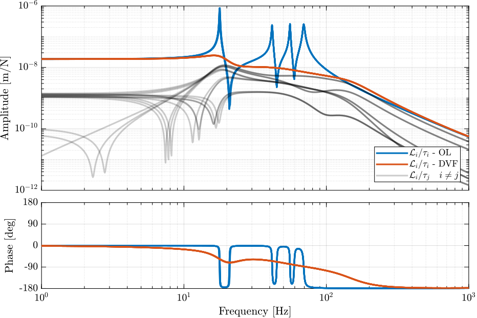
Figure 31: Bode plots of the transfer functions from actuator forces \(\tau_i\) to relative motion sensors \(\mathcal{L}_i\) with and without the DVF controller.

The Direct Velocity Feedback Strategy is very effective in damping the 6 suspension modes of the nano-hexapod.

4.4 Effect of DVF on the compliance

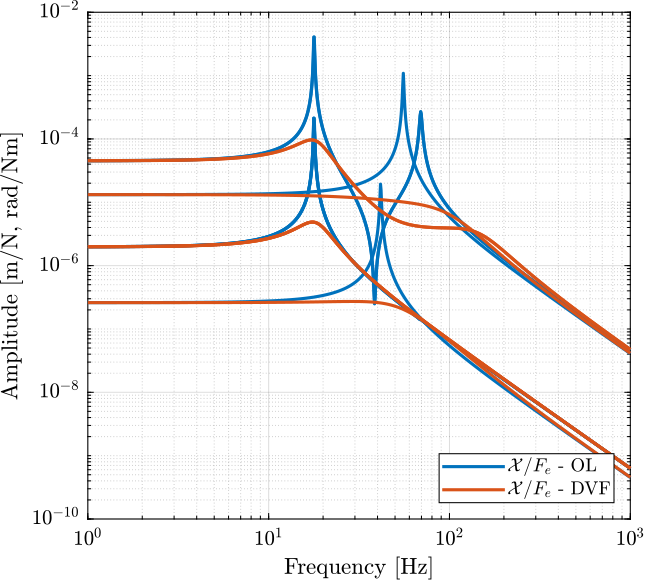
Figure 32: Comparison of the compliances in Open Loop and with Direct Velocity Feedback controller

5 Function - Initialize Nano Hexapod

Function description

function [nano_hexapod] = initializeNanoHexapodFinal(args)

Optional Parameters

arguments
    %% Bottom Flexible Joints
    args.flex_bot_type      char {mustBeMember(args.flex_bot_type,{'2dof', '3dof', '4dof', 'flexible'})} = '4dof'
    args.flex_bot_kRx (6,1) double {mustBeNumeric} = ones(6,1)*5 % X bending stiffness [Nm/rad]
    args.flex_bot_kRy (6,1) double {mustBeNumeric} = ones(6,1)*5 % Y bending stiffness [Nm/rad]
    args.flex_bot_kRz (6,1) double {mustBeNumeric} = ones(6,1)*260 % Torsionnal stiffness [Nm/rad]
    args.flex_bot_kz  (6,1) double {mustBeNumeric} = ones(6,1)*1e8 % Axial Stiffness [N/m]
    args.flex_bot_cRx (6,1) double {mustBeNumeric} = ones(6,1)*0.1 % X bending Damping [Nm/(rad/s)]
    args.flex_bot_cRy (6,1) double {mustBeNumeric} = ones(6,1)*0.1 % Y bending Damping [Nm/(rad/s)]
    args.flex_bot_cRz (6,1) double {mustBeNumeric} = ones(6,1)*0.1 % Torsionnal Damping [Nm/(rad/s)]
    args.flex_bot_cz  (6,1) double {mustBeNumeric} = ones(6,1)*1e2 % Axial Damping [N/(m/s)]
    %% Top Flexible Joints
    args.flex_top_type      char {mustBeMember(args.flex_top_type,{'2dof', '3dof', '4dof', 'flexible'})} = '4dof'
    args.flex_top_kRx (6,1) double {mustBeNumeric} = ones(6,1)*5 % X bending stiffness [Nm/rad]
    args.flex_top_kRy (6,1) double {mustBeNumeric} = ones(6,1)*5 % Y bending stiffness [Nm/rad]
    args.flex_top_kRz (6,1) double {mustBeNumeric} = ones(6,1)*260 % Torsionnal stiffness [Nm/rad]
    args.flex_top_kz  (6,1) double {mustBeNumeric} = ones(6,1)*1e8 % Axial Stiffness [N/m]
    args.flex_top_cRx (6,1) double {mustBeNumeric} = ones(6,1)*0.1 % X bending Damping [Nm/(rad/s)]
    args.flex_top_cRy (6,1) double {mustBeNumeric} = ones(6,1)*0.1 % Y bending Damping [Nm/(rad/s)]
    args.flex_top_cRz (6,1) double {mustBeNumeric} = ones(6,1)*0.1 % Torsionnal Damping [Nm/(rad/s)]
    args.flex_top_cz  (6,1) double {mustBeNumeric} = ones(6,1)*1e2 % Axial Damping [N/(m/s)]
    %% Jacobian - Location of frame {A} and {B}
    args.MO_B (1,1) double {mustBeNumeric} = 150e-3 % Height of {B} w.r.t. {M} [m]
    %% Relative Motion Sensor
    args.motion_sensor_type char {mustBeMember(args.motion_sensor_type,{'struts', 'plates'})} = 'struts'
    %% Actuators
    args.actuator_type char {mustBeMember(args.actuator_type,{'2dof', 'flexible frame', 'flexible'})} = 'flexible'
    args.actuator_Ga  (6,1) double {mustBeNumeric} = ones(6,1)*1 % Actuator gain [N/V]
    args.actuator_Gs  (6,1) double {mustBeNumeric} = ones(6,1)*1 % Sensor gain [V/m]
                                                                 % For 2DoF
    args.actuator_k   (6,1) double {mustBeNumeric} = ones(6,1)*0.35e6 % [N/m]
    args.actuator_ke  (6,1) double {mustBeNumeric} = ones(6,1)*1.5e6 % [N/m]
    args.actuator_ka  (6,1) double {mustBeNumeric} = ones(6,1)*43e6 % [N/m]
    args.actuator_c   (6,1) double {mustBeNumeric} = ones(6,1)*3e1 % [N/(m/s)]
    args.actuator_ce  (6,1) double {mustBeNumeric} = ones(6,1)*1e1 % [N/(m/s)]
    args.actuator_ca  (6,1) double {mustBeNumeric} = ones(6,1)*1e1 % [N/(m/s)]
    args.actuator_Leq (6,1) double {mustBeNumeric} = ones(6,1)*0.056 % [m]
                                                                     % For Flexible Frame
    args.actuator_ks (6,1) double {mustBeNumeric} = ones(6,1)*235e6 % Stiffness of one stack [N/m]
    args.actuator_cs (6,1) double {mustBeNumeric} = ones(6,1)*1e1 % Stiffness of one stack [N/m]

    args.actuator_xi  (1,1) double {mustBeNumeric} = 0.01 % Damping Ratio
    %% Controller
    args.controller_type char {mustBeMember(args.controller_type,{'none', 'iff', 'dvf'})} = 'none'
end

Nano Hexapod Object

nano_hexapod = struct();

Flexible Joints - Bot

nano_hexapod.flex_bot = struct();

switch args.flex_bot_type
  case '2dof'
    nano_hexapod.flex_bot.type = 1;
  case '3dof'
    nano_hexapod.flex_bot.type = 2;
  case '4dof'
    nano_hexapod.flex_bot.type = 3;
  case 'flexible'
    nano_hexapod.flex_bot.type = 4;
end

nano_hexapod.flex_bot.kRx = args.flex_bot_kRx; % X bending stiffness [Nm/rad]
nano_hexapod.flex_bot.kRy = args.flex_bot_kRy; % Y bending stiffness [Nm/rad]
nano_hexapod.flex_bot.kRz = args.flex_bot_kRz; % Torsionnal stiffness [Nm/rad]
nano_hexapod.flex_bot.kz  = args.flex_bot_kz;  % Axial stiffness [N/m]

nano_hexapod.flex_bot.cRx = args.flex_bot_cRx; % [Nm/(rad/s)]
nano_hexapod.flex_bot.cRy = args.flex_bot_cRy; % [Nm/(rad/s)]
nano_hexapod.flex_bot.cRz = args.flex_bot_cRz; % [Nm/(rad/s)]
nano_hexapod.flex_bot.cz  = args.flex_bot_cz;  %[N/(m/s)]

Flexible Joints - Top

nano_hexapod.flex_top = struct();

switch args.flex_top_type
  case '2dof'
    nano_hexapod.flex_top.type = 1;
  case '3dof'
    nano_hexapod.flex_top.type = 2;
  case '4dof'
    nano_hexapod.flex_top.type = 3;
  case 'flexible'
    nano_hexapod.flex_top.type = 4;
end

nano_hexapod.flex_top.kRx = args.flex_top_kRx; % X bending stiffness [Nm/rad]
nano_hexapod.flex_top.kRy = args.flex_top_kRy; % Y bending stiffness [Nm/rad]
nano_hexapod.flex_top.kRz = args.flex_top_kRz; % Torsionnal stiffness [Nm/rad]
nano_hexapod.flex_top.kz  = args.flex_top_kz;  % Axial stiffness [N/m]

nano_hexapod.flex_top.cRx = args.flex_top_cRx; % [Nm/(rad/s)]
nano_hexapod.flex_top.cRy = args.flex_top_cRy; % [Nm/(rad/s)]
nano_hexapod.flex_top.cRz = args.flex_top_cRz; % [Nm/(rad/s)]
nano_hexapod.flex_top.cz  = args.flex_top_cz;  %[N/(m/s)]

Relative Motion Sensor

nano_hexapod.motion_sensor = struct();

switch args.motion_sensor_type
  case 'struts'
    nano_hexapod.motion_sensor.type = 1;
  case 'plates'
    nano_hexapod.motion_sensor.type = 2;
end

Amplified Piezoelectric Actuator

nano_hexapod.actuator = struct();

switch args.actuator_type
  case '2dof'
    nano_hexapod.actuator.type = 1;
  case 'flexible frame'
    nano_hexapod.actuator.type = 2;
  case 'flexible'
    nano_hexapod.actuator.type = 3;
end

nano_hexapod.actuator.Ga = args.actuator_Ga; % Actuator gain [N/V]
nano_hexapod.actuator.Gs = args.actuator_Gs; % Sensor gain [V/m]

2dof

nano_hexapod.actuator.k  = args.actuator_k;  % [N/m]
nano_hexapod.actuator.ke = args.actuator_ke; % [N/m]
nano_hexapod.actuator.ka = args.actuator_ka; % [N/m]

nano_hexapod.actuator.c  = args.actuator_c;  % [N/(m/s)]
nano_hexapod.actuator.ce = args.actuator_ce; % [N/(m/s)]
nano_hexapod.actuator.ca = args.actuator_ca; % [N/(m/s)]

nano_hexapod.actuator.Leq = args.actuator_Leq; % [m]

Flexible frame and fully flexible

switch args.actuator_type
  case 'flexible frame'
    nano_hexapod.actuator.K = readmatrix('APA300ML_b_mat_K.CSV'); % Stiffness Matrix
    nano_hexapod.actuator.M = readmatrix('APA300ML_b_mat_M.CSV'); % Mass Matrix
    nano_hexapod.actuator.P = extractNodes('APA300ML_b_out_nodes_3D.txt'); % Node coordinates [m]
  case 'flexible'
    nano_hexapod.actuator.K = readmatrix('full_APA300ML_K.CSV'); % Stiffness Matrix
    nano_hexapod.actuator.M = readmatrix('full_APA300ML_M.CSV'); % Mass Matrix
    nano_hexapod.actuator.P = extractNodes('full_APA300ML_out_nodes_3D.txt'); % Node coordiantes [m]
end

nano_hexapod.actuator.xi = args.actuator_xi; % Damping ratio

nano_hexapod.actuator.ks = args.actuator_ks; % Stiffness of one stack [N/m]
nano_hexapod.actuator.cs = args.actuator_cs; % Damping of one stack [N/m]

Geometry

nano_hexapod.geometry = struct();

Center of joints \(a_i\) with respect to {F}:

Fa = [[-86.05,  -74.78, 22.49],
      [ 86.05,  -74.78, 22.49],
      [ 107.79, -37.13, 22.49],
      [ 21.74,  111.91, 22.49],
      [-21.74,  111.91, 22.49],
      [-107.79, -37.13, 22.49]]'*1e-3; % Ai w.r.t. {F} [m]

Center of joints \(b_i\) with respect to {M}:

Mb = [[-28.47, -106.25, -22.50],
      [ 28.47, -106.25, -22.50],
      [ 106.25, 28.47,  -22.50],
      [ 77.78,  77.78,  -22.50],
      [-77.78,  77.78,  -22.50],
      [-106.25, 28.47,  -22.50]]'*1e-3; % Bi w.r.t. {M} [m]

Now compute the positions \(b_i\) with respect to {F}:

Fb = Mb + [0; 0; 95e-3]; % Bi w.r.t. {F} [m]

The unit vector representing the orientation of the struts can then be computed:

si = Fb - Fa;
si = si./vecnorm(si); % Normalize

Location of encoder measurement points when fixed on the plates:

Fc = [[-29.362, -105.765, 52.605]
      [ 29.362, -105.765, 52.605]
      [ 106.276, 27.454,  52.605]
      [ 76.914,  78.31,   52.605]
      [-76.914,  78.31,   52.605]
      [-106.276, 27.454,  52.605]]'*1e-3; % Meas pos w.r.t. {F}
Mc = Fc - [0; 0; 95e-3]; % Meas pos w.r.t. {M}

nano_hexapod.geometry.Fa = Fa;
nano_hexapod.geometry.Fb = Fb;
nano_hexapod.geometry.Fc = Fc;
nano_hexapod.geometry.Mb = Mb;
nano_hexapod.geometry.Mc = Mc;
nano_hexapod.geometry.si = si;
nano_hexapod.geometry.MO_B = args.MO_B;

Jacobian for Actuators

Bb = Mb - [0; 0; args.MO_B];

nano_hexapod.geometry.J = [nano_hexapod.geometry.si', cross(Bb, nano_hexapod.geometry.si)'];

Jacobian for Sensors

switch args.motion_sensor_type
  case 'struts'
    nano_hexapod.geometry.Js = nano_hexapod.geometry.J;
  case 'plates'
    Bc = Mc - [0; 0; args.MO_B];
    nano_hexapod.geometry.Js = [nano_hexapod.geometry.si', cross(Bc, nano_hexapod.geometry.si)'];
end

Controller

switch args.controller_type
  case 'none'
    nano_hexapod.controller.type = 1;
  case 'iff'
    nano_hexapod.controller.type = 2;
  case 'dvf'
    nano_hexapod.controller.type = 3;
end

Save the Structure

if nargout == 0
  save('./mat/stages.mat', 'nano_hexapod', '-append');
end

Nano-Hexapod

Table of Contents

1 Nano-Hexapod

1.1 Nano Hexapod - Configuration

1.1.1 Flexible Joints

1.1.2 Amplified Piezoelectric Actuators

1.1.3 Encoders

1.1.4 Jacobians

1.2 Effect of encoders on the decentralized plant

1.3 Effect of APA flexibility

1.4 Nano Hexapod - Number of DoF

1.5 Direct Velocity Feedback Plant

1.6 Integral Force Feedback Plant

1.7 Decentralized Plant - Cartesian coordinates

1.7.1 Verification of the Sensor Jacobian

1.7.2 Comparison of the decentralized plants

1.8 Decentralized Plant - Decoupling at the Center of Stiffness

1.8.1 Center of Stiffness

1.8.2 Obtained plant

1.9 Stiffness matrix

1.9.1 Compute the theoretical stiffness of the nano-hexapod

1.9.2 Comparison with Simscape Model

2 Active Damping using Integral Force Feedback

2.1 Plant Identification

2.2 Root Locus

2.3 Effect of IFF on the plant

2.4 Effect of IFF on the compliance

3 Active Damping using Direct Velocity Feedback - Encoders on the struts

3.1 Plant Identification

3.2 Root Locus

3.3 Effect of DVF on the plant

3.4 Effect of DVF on the compliance

4 Active Damping using Direct Velocity Feedback - Encoders on the plates

4.1 Plant Identification

4.2 Root Locus

4.3 Effect of DVF on the plant

4.4 Effect of DVF on the compliance

5 Function - Initialize Nano Hexapod

Function description

Optional Parameters

Nano Hexapod Object

Flexible Joints - Bot

Flexible Joints - Top

Relative Motion Sensor

Amplified Piezoelectric Actuator

Geometry

Jacobian for Actuators

Jacobian for Sensors

Controller

Save the Structure