HAC-LAC applied on the Simscape Model

1. Initialization
2. Low Authority Control - Direct Velocity Feedback \(\bm{K}_\mathcal{L}\)
3. Uncertainty Improvements thanks to the LAC control
4. High Authority Control - \(\bm{K}_\mathcal{X}\)
- 4.1. Identification of the damped plant
- 4.2. Controller Design
5. Simulation
6. Results

The position \(\bm{\mathcal{X}}\) of the Sample with respect to the granite is measured.

It is then compare to the wanted position of the Sample \(\bm{r}_\mathcal{X}\) in order to obtain the position error \(\bm{\epsilon}_\mathcal{X}\) of the Sample with respect to a frame attached to the Stewart top platform.

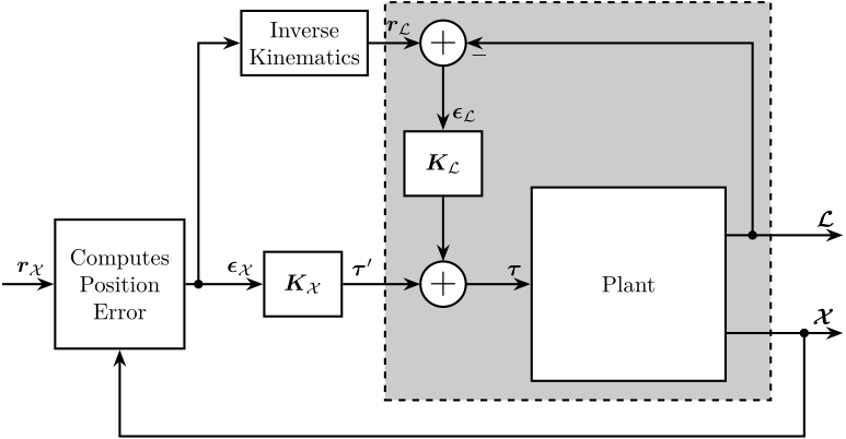
Figure 1: HAC-LAC Control Architecture used for the Control of the NASS

1 Initialization

We initialize all the stages with the default parameters.

initializeGround();
initializeGranite();
initializeTy();
initializeRy();
initializeRz();
initializeMicroHexapod();
initializeAxisc();
initializeMirror();

The nano-hexapod is a piezoelectric hexapod and the sample has a mass of 50kg.

initializeNanoHexapod('actuator', 'piezo');
initializeSample('mass', 1);

We set the references that corresponds to a tomography experiment.

initializeReferences('Rz_type', 'rotating', 'Rz_period', 1);

initializeDisturbances();

Open Loop.

initializeController('type', 'open-loop');

And we put some gravity.

initializeSimscapeConfiguration('gravity', true);

We log the signals.

initializeLoggingConfiguration('log', 'all');

2 Low Authority Control - Direct Velocity Feedback \(\bm{K}_\mathcal{L}\)

The first loop closed corresponds to a direct velocity feedback loop.

The design of the associated decentralized controller is explained in this file.

2.1 Identification

%% Name of the Simulink File
mdl = 'nass_model';

%% Input/Output definition
clear io; io_i = 1;
io(io_i) = linio([mdl, '/Controller'],    1, 'openinput');               io_i = io_i + 1; % Actuator Inputs
io(io_i) = linio([mdl, '/Micro-Station'], 3, 'openoutput', [], 'Dnlm');  io_i = io_i + 1; % Relative Motion Outputs

%% Run the linearization
G_dvf = linearize(mdl, io, 0);
G_dvf.InputName  = {'Fnl1', 'Fnl2', 'Fnl3', 'Fnl4', 'Fnl5', 'Fnl6'};
G_dvf.OutputName = {'Dnlm1', 'Dnlm2', 'Dnlm3', 'Dnlm4', 'Dnlm5', 'Dnlm6'};

2.2 Plant

2.3 Root Locus

2.4 Controller and Loop Gain

K_dvf = s*15000/(1 + s/2/pi/10000);

K_dvf = -K_dvf*eye(6);

3 Uncertainty Improvements thanks to the LAC control

K_dvf_backup = K_dvf;
initializeController('type', 'hac-dvf');

masses = [1, 10, 50]; % [kg]

%% Name of the Simulink File
mdl = 'nass_model';

%% Input/Output definition
clear io; io_i = 1;
io(io_i) = linio([mdl, '/Controller'],     1, 'input');            io_i = io_i + 1; % Actuator Inputs
io(io_i) = linio([mdl, '/Tracking Error'], 1, 'output', [], 'En'); io_i = io_i + 1; % Position Errror

4 High Authority Control - \(\bm{K}_\mathcal{X}\)

4.1 Identification of the damped plant

Kx = tf(zeros(6));

initializeController('type', 'hac-dvf');

%% Name of the Simulink File
mdl = 'nass_model';

%% Input/Output definition
clear io; io_i = 1;
io(io_i) = linio([mdl, '/Controller'],     1, 'input');            io_i = io_i + 1; % Actuator Inputs
io(io_i) = linio([mdl, '/Tracking Error'], 1, 'output', [], 'En'); io_i = io_i + 1; % Position Errror

%% Run the linearization
G = linearize(mdl, io, 0);
G.InputName  = {'Fnl1', 'Fnl2', 'Fnl3', 'Fnl4', 'Fnl5', 'Fnl6'};
G.OutputName = {'Ex', 'Ey', 'Ez', 'Erx', 'Ery', 'Erz'};

The minus sine is put here because there is already a minus sign included due to the computation of the position error.

load('mat/stages.mat', 'nano_hexapod');

Gx = -G*inv(nano_hexapod.kinematics.J');
Gx.InputName  = {'Fx', 'Fy', 'Fz', 'Mx', 'My', 'Mz'};

4.2 Controller Design

The controller consists of:

A pure integrator
A Second integrator up to half the wanted bandwidth
A Lead around the cross-over frequency
A low pass filter with a cut-off equal to two times the wanted bandwidth

wc = 2*pi*15; % Bandwidth Bandwidth [rad/s]

h = 1.5; % Lead parameter

Kx = (1/h) * (1 + s/wc*h)/(1 + s/wc/h) * wc/s * ((s/wc*2 + 1)/(s/wc*2)) * (1/(1 + s/wc/2));

% Normalization of the gain of have a loop gain of 1 at frequency wc
Kx = Kx.*diag(1./diag(abs(freqresp(Gx*Kx, wc))));

isstable(feedback(Gx*Kx, eye(6), -1))

Kx = inv(nano_hexapod.kinematics.J')*Kx;

isstable(feedback(G*Kx, eye(6), 1))

5 Simulation

load('mat/conf_simulink.mat');
set_param(conf_simulink, 'StopTime', '2');

And we simulate the system.

sim('nass_model');

hac_dvf = simout;
save('./mat/tomo_exp_hac_lac.mat', 'hac_dvf');

6 Results

Let’s load the simulation when no control is applied.

load('./mat/experiment_tomography.mat', 'tomo_align_dist');
load('./mat/tomo_exp_hac_lac.mat', 'hac_dvf');