Active Damping applied on the Simscape Model

1. Undamped System
2. Variability of the system dynamics for Active Damping
3. Integral Force Feedback
4. Direct Velocity Feedback
5. Inertial Control
- 5.1. Control Design
- 5.2. Conclusion
6. Comparison
7. Useful Functions
- 7.1. prepareLinearizeIdentification
- 7.2. prepareTomographyExperiment

The goal of this file is to study the use of active damping for the control of the NASS.

In general, three sensors can be used for Active Damping:

A force sensor
A relative motion sensor such as a capacitive sensor
An inertial sensor such as an accelerometer of geophone

First, in section 1, we look at the undamped system and we identify the dynamics from the actuators to the three sensor types.

Then, in section 2, we study the change of dynamics for the active damping plants with respect to various experimental conditions such as the sample mass and the spindle rotation speed.

Then, we will apply and compare the results of three active damping techniques:

In section 3: Integral Force Feedback is applied
In section 4: Direct Velocity Feedback using a relative motion sensor is applied
In section 5: Inertial Control using a geophone is applied

For each of the active damping technique, we:

Look at the obtain damped plant that will be used for High Authority control
Simulate tomography experiments
Compare the sensitivity from disturbances

1 Undamped System

In this section, we identify the dynamic of the system from forces applied in the nano-hexapod legs to the various sensors included in the nano-hexapod that could be use for Active Damping, namely:

A relative motion sensor, measuring the relative displacement of each of the leg
A force sensor measuring the total force transmitted to the top part of the leg in the direction of the leg
A absolute velocity sensor measuring the absolute velocity of the top part of the leg in the direction of the leg

After that, a tomography experiment is simulation without any active damping techniques.

1.1 Identification of the dynamics for Active Damping

1.1.1 Identification

We initialize all the stages with the default parameters.

prepareLinearizeIdentification();

We identify the dynamics of the system using the linearize function.

%% Options for Linearized
options = linearizeOptions;
options.SampleTime = 0;

%% Name of the Simulink File
mdl = 'nass_model';

%% Input/Output definition
clear io; io_i = 1;
io(io_i) = linio([mdl, '/Controller'],    1, 'openinput');               io_i = io_i + 1; % Actuator Inputs
io(io_i) = linio([mdl, '/Micro-Station'], 3, 'openoutput', [], 'Dnlm');  io_i = io_i + 1; % Relative Motion Outputs
io(io_i) = linio([mdl, '/Micro-Station'], 3, 'openoutput', [], 'Fnlm');  io_i = io_i + 1; % Force Sensors
io(io_i) = linio([mdl, '/Micro-Station'], 3, 'openoutput', [], 'Vlm');   io_i = io_i + 1; % Absolute Velocity Outputs

%% Run the linearization
G = linearize(mdl, io, 0.5, options);
G.InputName  = {'Fnl1', 'Fnl2', 'Fnl3', 'Fnl4', 'Fnl5', 'Fnl6'};
G.OutputName = {'Dnlm1', 'Dnlm2', 'Dnlm3', 'Dnlm4', 'Dnlm5', 'Dnlm6', ...
                'Fnlm1', 'Fnlm2', 'Fnlm3', 'Fnlm4', 'Fnlm5', 'Fnlm6', ...
                'Vnlm1', 'Vnlm2', 'Vnlm3', 'Vnlm4', 'Vnlm5', 'Vnlm6'};

We then create transfer functions corresponding to the active damping plants.

G_iff = minreal(G({'Fnlm1', 'Fnlm2', 'Fnlm3', 'Fnlm4', 'Fnlm5', 'Fnlm6'}, {'Fnl1', 'Fnl2', 'Fnl3', 'Fnl4', 'Fnl5', 'Fnl6'}));
G_dvf = minreal(G({'Dnlm1', 'Dnlm2', 'Dnlm3', 'Dnlm4', 'Dnlm5', 'Dnlm6'}, {'Fnl1', 'Fnl2', 'Fnl3', 'Fnl4', 'Fnl5', 'Fnl6'}));
G_ine = minreal(G({'Vnlm1', 'Vnlm2', 'Vnlm3', 'Vnlm4', 'Vnlm5', 'Vnlm6'}, {'Fnl1', 'Fnl2', 'Fnl3', 'Fnl4', 'Fnl5', 'Fnl6'}));

And we save them for further analysis.

save('./mat/active_damping_undamped_plants.mat', 'G_iff', 'G_dvf', 'G_ine');

1.1.2 Obtained Plants for Active Damping

load('./mat/active_damping_undamped_plants.mat', 'G_iff', 'G_dvf', 'G_ine');

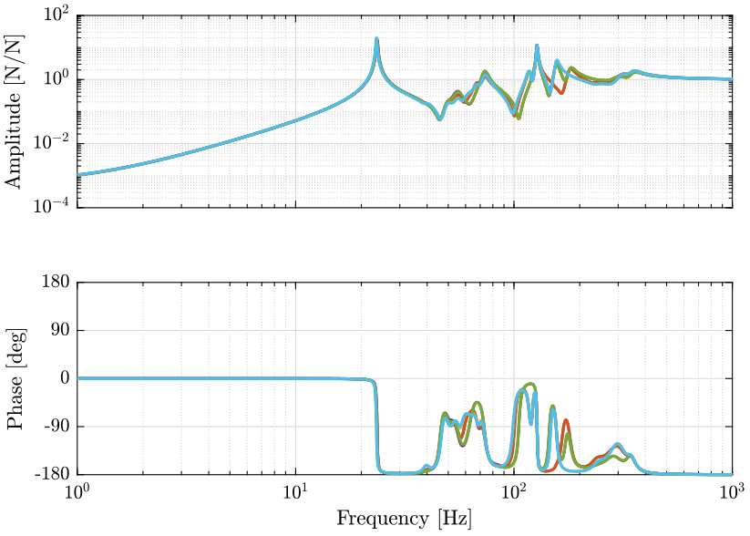
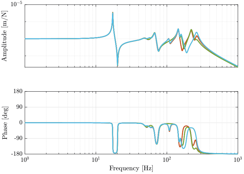
Figure 1: G_iff: Transfer functions from forces applied in the actuators to the force sensor in each actuator (png, pdf)

Figure 2: G_dvf: Transfer functions from forces applied in the actuators to the relative motion sensor in each actuator (png, pdf)

Figure 3: G_ine: Transfer functions from forces applied in the actuators to the geophone located in each leg measuring the absolute velocity of the top part of the leg in the direction of the leg (png, pdf)

1.2 Identification of the dynamics for High Authority Control

1.2.1 Identification

We initialize all the stages with the default parameters.

prepareLinearizeIdentification();

We identify the dynamics of the system using the linearize function.

%% Options for Linearized
options = linearizeOptions;
options.SampleTime = 0;

%% Name of the Simulink File
mdl = 'nass_model';

%% Input/Output definition
clear io; io_i = 1;
io(io_i) = linio([mdl, '/Controller'],     1, 'openinput');            io_i = io_i + 1; % Actuator Inputs
io(io_i) = linio([mdl, '/Tracking Error'], 1, 'openoutput', [], 'En'); io_i = io_i + 1; % Metrology Outputs

masses = [1, 10, 50]; % [kg]

And we save them for further analysis.

save('./mat/active_damping_cart_plants.mat', 'G_cart', 'masses');

1.2.2 Obtained Plants

load('./mat/active_damping_cart_plants.mat', 'G_cart', 'masses');

Figure 4: Undamped Plant - Translations (png, pdf)

Figure 5: Undamped Plant - Rotations (png, pdf)

1.3 Tomography Experiment

1.3.1 Simulation

We initialize elements for the tomography experiment.

prepareTomographyExperiment();

We change the simulation stop time.

load('mat/conf_simulink.mat');
set_param(conf_simulink, 'StopTime', '4.5');

And we simulate the system.

sim('nass_model');

Finally, we save the simulation results for further analysis

save('./mat/active_damping_tomo_exp.mat', 'En', 'Eg', '-append');

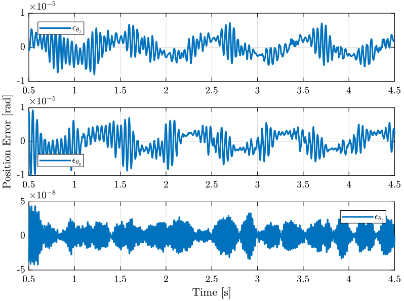
1.3.2 Results

We load the results of tomography experiments.

load('./mat/active_damping_tomo_exp.mat', 'En');
Fs = 1e3; % Sampling Frequency of the Data
t = (1/Fs)*[0:length(En(:,1))-1];

Figure 6: Position Error during tomography experiment - Translations (png, pdf)

Figure 7: Position Error during tomography experiment - Rotations (png, pdf)

2 Variability of the system dynamics for Active Damping

The goal of this section is to study how the dynamics of the Active Damping plants are changing with the experimental conditions. These experimental conditions are:

The mass of the sample (section 2.1)
The spindle angle with a null rotating speed (section 2.2)
The spindle rotation speed (section 2.3)
The tilt angle (section 2.4)
The scans of the translation stage (section 2.5)

For the identification of the dynamics, the system is simulation for \(\approx 0.5s\) before the linearization is performed. This is done in order for the transient phase to be over.

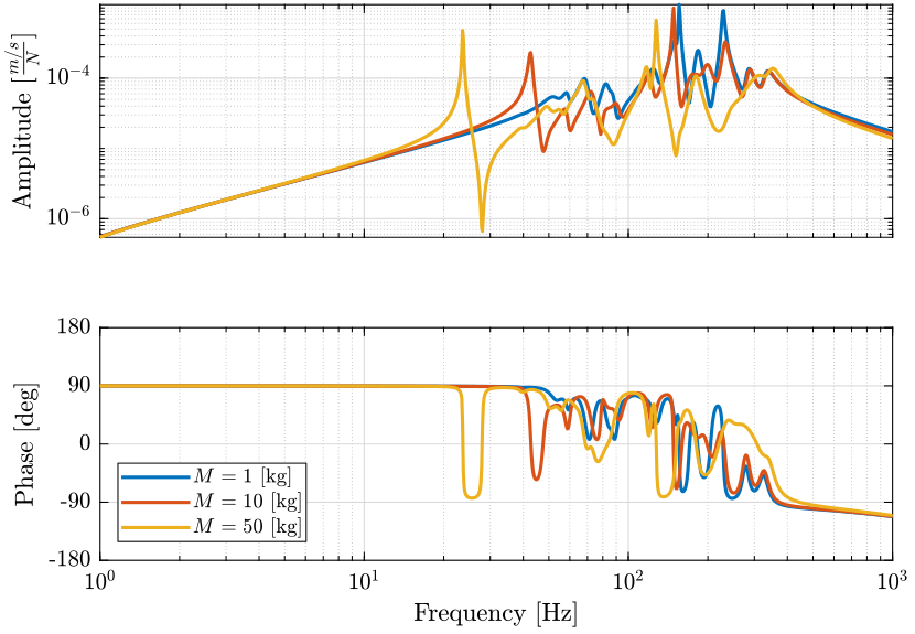
2.1 Variation of the Sample Mass

For all the identifications, the disturbances are disabled and no controller are used.

We initialize all the stages with the default parameters.

prepareLinearizeIdentification();

We identify the dynamics for the following sample mass.

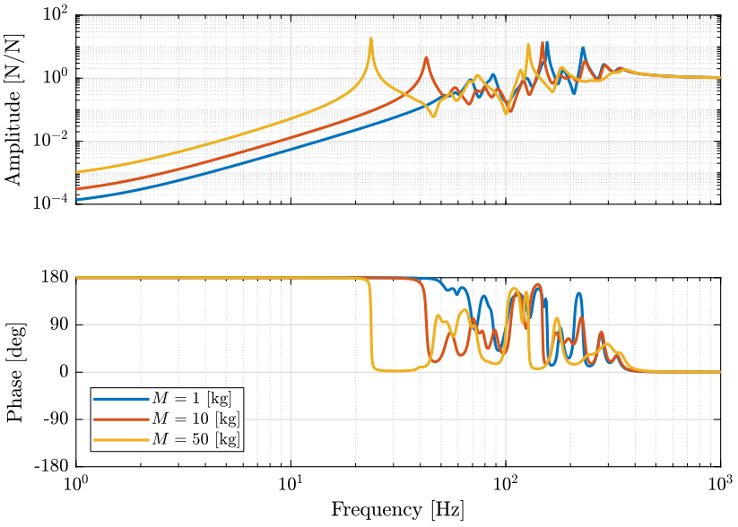
masses = [1, 10, 50]; % [kg]

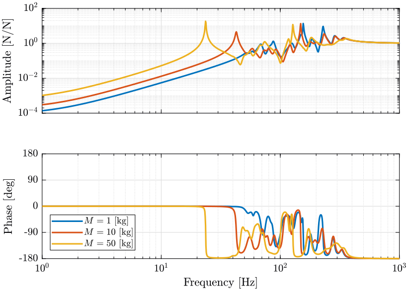
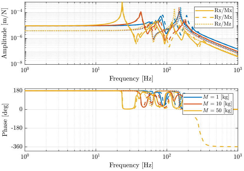
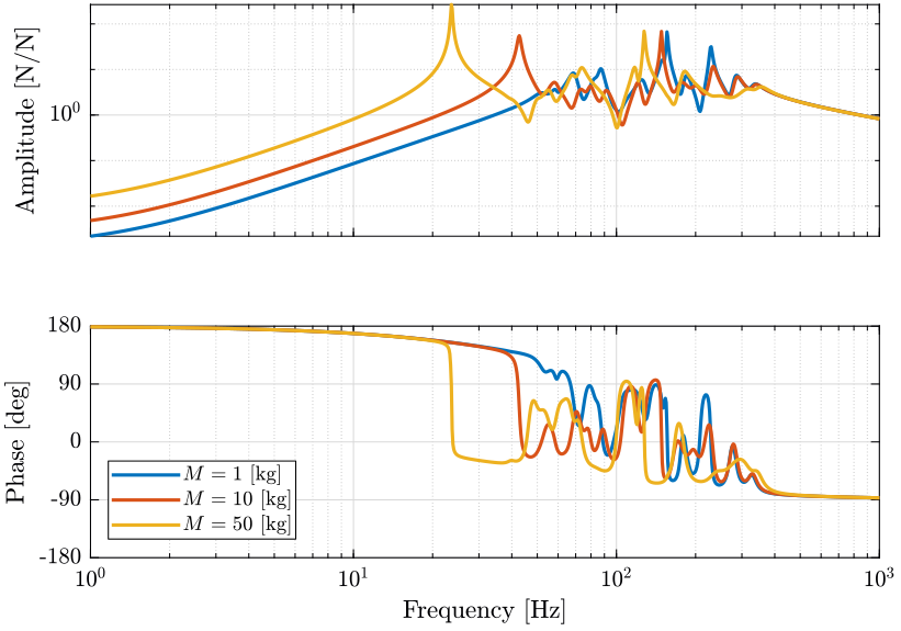
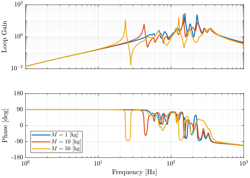
Figure 8: Variability of the dynamics from actuator force to force sensor with the Sample Mass (png, pdf)

Figure 9: Variability of the dynamics from actuator force to relative motion sensor with the Sample Mass (png, pdf)

Figure 10: Variability of the dynamics from actuator force to absolute velocity with the Sample Mass (png, pdf)

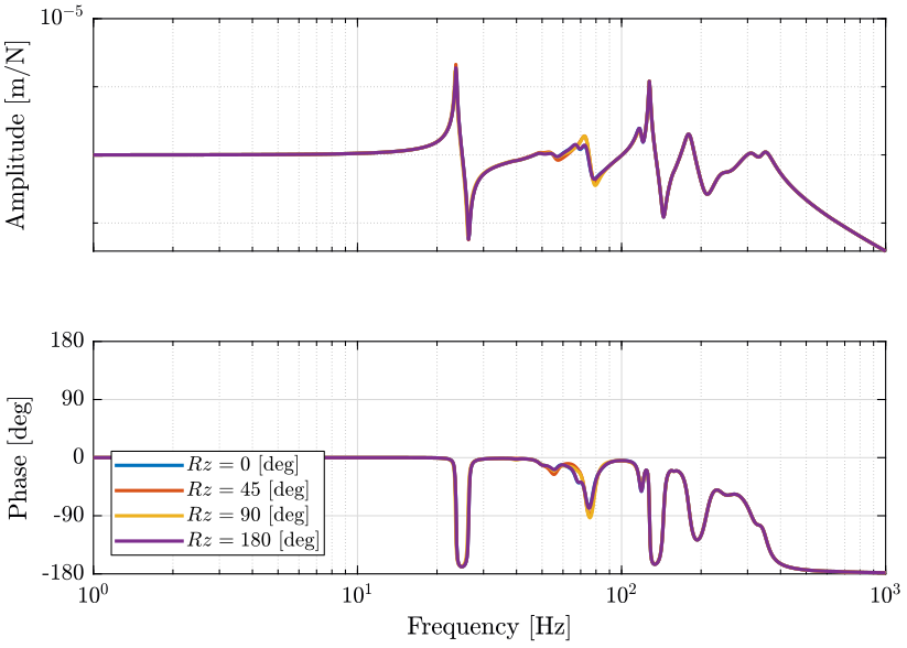
2.2 Variation of the Spindle Angle

We initialize all the stages with the default parameters.

prepareLinearizeIdentification();

We identify the dynamics for the following Spindle angles.

Rz_amplitudes = [0, pi/4, pi/2, pi]; % [rad]

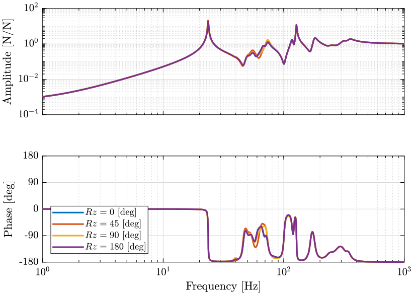
Figure 11: Variability of the dynamics from the actuator force to the force sensor with the Spindle Angle (png, pdf)

Figure 12: Variability of the dynamics from actuator force to relative motion sensor with the Spindle Angle (png, pdf)

Figure 13: Variability of the dynamics from actuator force to absolute velocity with the Spindle Angle (png, pdf)

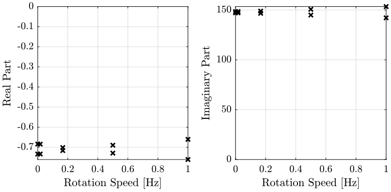
2.3 Variation of the Spindle Rotation Speed

We initialize all the stages with the default parameters.

prepareLinearizeIdentification();

We identify the dynamics for the following Spindle rotation periods.

Rz_periods = [60, 6, 2, 1]; % [s]

The identification of the dynamics is done at the same Spindle angle position.

2.3.1 Dynamics of the Active Damping plants

Figure 14: Variability of the dynamics from the actuator force to the force sensor with the Spindle rotation speed (png, pdf)

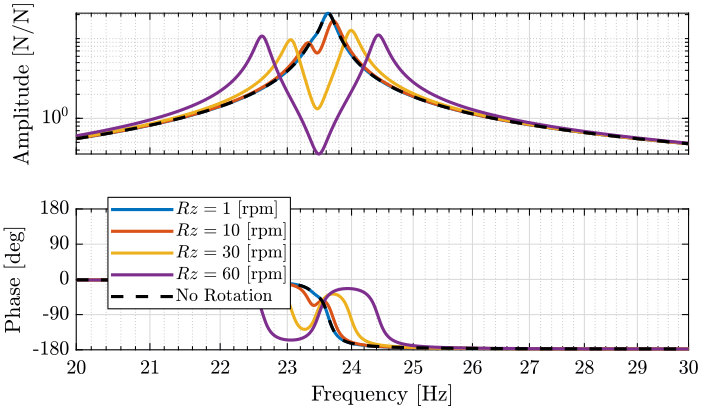
Figure 15: Variability of the dynamics from the actuator force to the force sensor with the Spindle rotation speed (png, pdf)

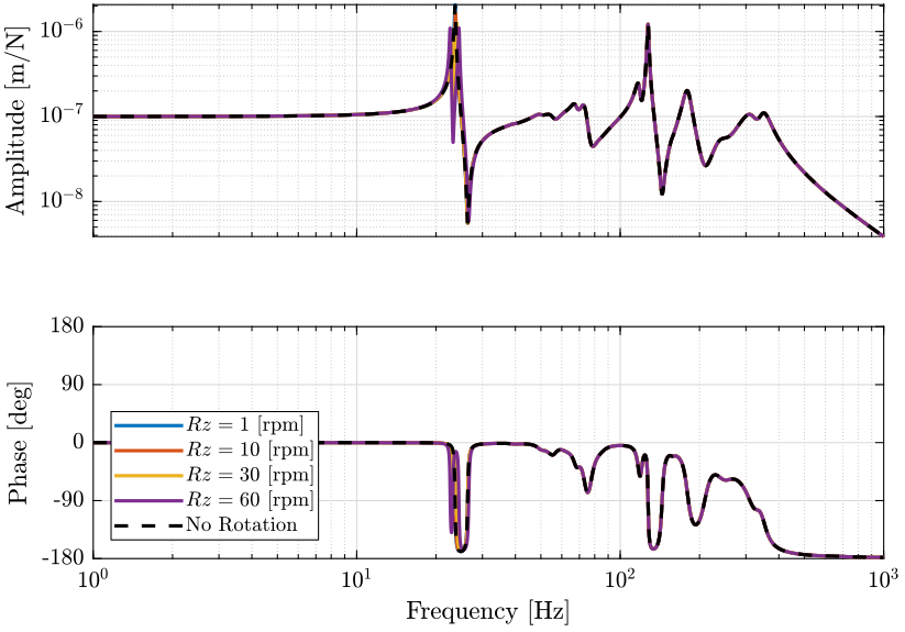
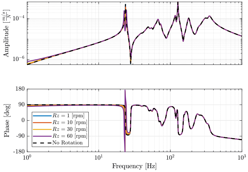
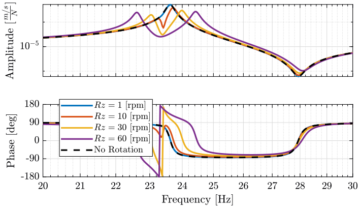
Figure 16: Variability of the dynamics from the actuator force to the relative motion sensor with the Spindle rotation speed (png, pdf)

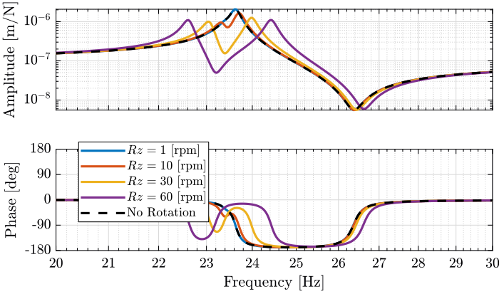
Figure 17: Variability of the dynamics from the actuator force to the relative motion sensor with the Spindle rotation speed (png, pdf)

Figure 18: Variability of the dynamics from the actuator force to the absolute velocity sensor with the Spindle rotation speed (png, pdf)

Figure 19: Variability of the dynamics from the actuator force to the absolute velocity sensor with the Spindle rotation speed (png, pdf)

2.3.2 Variation of the poles and zeros with the Spindle rotation frequency

Figure 20: Evolution of the pole with respect to the spindle rotation speed (png, pdf)

Figure 21: Evolution of the zero with respect to the spindle rotation speed (png, pdf)

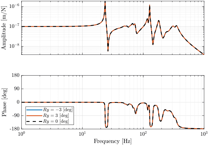
2.4 Variation of the Tilt Angle

We initialize all the stages with the default parameters.

prepareLinearizeIdentification();

We identify the dynamics for the following Tilt stage angles.

Ry_amplitudes = [-3*pi/180, 3*pi/180]; % [rad]

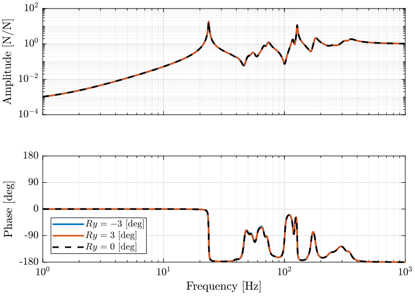
Figure 22: Variability of the dynamics from the actuator force to the force sensor with the Tilt stage Angle (png, pdf)

Figure 23: Variability of the dynamics from the actuator force to the relative motion sensor with the Tilt Angle (png, pdf)

Figure 24: Variability of the dynamics from the actuator force to the absolute velocity sensor with the Tilt Angle (png, pdf)

2.5 Scans of the Translation Stage

We want here to verify if the dynamics used for Active damping is varying when using the translation stage for scans.

We initialize all the stages with the default parameters.

prepareLinearizeIdentification();

We initialize the translation stage reference to be a sinus with an amplitude of 5mm and a period of 1s (Figure 25).

initializeReferences('Dy_type', 'sinusoidal', ...
                     'Dy_amplitude', 5e-3, ... % [m]
                     'Dy_period', 1); % [s]

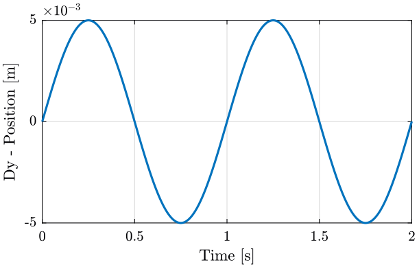
Figure 25: Reference path for the translation stage (png, pdf)

We identify the dynamics at different positions (times) when scanning with the Translation stage.

t_lin = [0.5, 0.75, 1, 1.25];

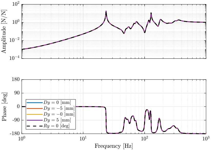
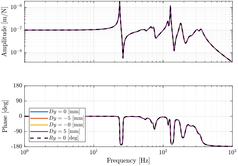
Figure 26: Variability of the dynamics from the actuator force to the absolute velocity sensor plant at different Ty scan positions (png, pdf)

Figure 27: Variability of the dynamics from actuator force to relative displacement sensor at different Ty scan positions (png, pdf)

Figure 28: Variability of the Inertial plant at different Ty scan positions (png, pdf)

2.6 Conclusion

Table 1: Conclusion on the variability of the system dynamics for active damping
	Change of Dynamics
Sample Mass	Large
Spindle Angle	Small
Spindle Rotation Speed	First resonance is split in two resonances
Tilt Angle	Negligible
Translation Stage scans	Negligible

Also, for the Inertial Sensor, a RHP zero may appear when the spindle is rotating fast.

When using either a force sensor or a relative motion sensor for active damping, the only “parameter” that induce a large change for the dynamics to be controlled is the sample mass. Thus, the developed damping techniques should be robust to variations of the sample mass.

3 Integral Force Feedback

All the files (data and Matlab scripts) are accessible here.

Here, we study the use of Integral Force Feedback (IFF) to actively damp the resonances.

The IFF control is applied in a decentralized way: there is on controller for each leg.

The control architecture is represented in figure 29 where one of the 6 nano-hexapod legs is represented.

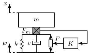
Figure 29: Integral Force Feedback applied to a 1dof system

3.1 Control Design

3.1.1 Plant

Let’s load the previously identified undamped plant:

load('./mat/active_damping_undamped_plants.mat', 'G_iff');
load('./mat/active_damping_plants_variable.mat', 'masses', 'Gm_iff');

Let’s look at the transfer function from actuator forces in the nano-hexapod to the force sensor in the nano-hexapod legs for all 6 pairs of actuator/sensor (figure 30).

Figure 30: Transfer function from forces applied in the legs to force sensor (png, pdf)

3.1.2 Control Design

The controller for each pair of actuator/sensor is:

w0 = 2*pi*50;
K_iff = -5000/s * (s/w0)/(1 + s/w0);

The corresponding loop gains are shown in figure 31.

Figure 31: Loop Gain for the Integral Force Feedback (png, pdf)

3.1.3 Diagonal Controller

We create the diagonal controller and we add a minus sign as we have a positive feedback architecture.

K_iff = -K_iff*eye(6);

We save the controller for further analysis.

save('./mat/active_damping_K_iff.mat', 'K_iff');

3.2 Tomography Experiment

3.2.1 Simulation with IFF Controller

We initialize elements for the tomography experiment.

prepareTomographyExperiment();

We set the IFF controller.

load('./mat/active_damping_K_iff.mat', 'K_iff');
initializeController('type', 'iff');

We change the simulation stop time.

load('mat/conf_simulink.mat');
set_param(conf_simulink, 'StopTime', '4.5');

And we simulate the system.

sim('nass_model');

Finally, we save the simulation results for further analysis

En_iff = En;
Eg_iff = Eg;
save('./mat/active_damping_tomo_exp.mat', 'En_iff', 'Eg_iff', '-append');

3.2.2 Compare with Undamped system

Figure 32: Position Error during tomography experiment - XY Motion (png, pdf)

Figure 33: Position Error during tomography experiment - Translations (png, pdf)

Figure 34: Position Error during tomography experiment - Rotations (png, pdf)

3.3 Conclusion

Integral Force Feedback using a force sensor:

Robust (guaranteed stability)
Acceptable Damping
Increase the sensitivity to disturbances at low frequencies

4 Direct Velocity Feedback

All the files (data and Matlab scripts) are accessible here.

In the Direct Velocity Feedback (DVF), a derivative feedback is applied between the measured actuator displacement to the actuator force input. The actuator displacement can be measured with a capacitive sensor for instance.

4.1 Control Design

4.1.1 Plant

Let’s load the undamped plant:

load('./mat/active_damping_undamped_plants.mat', 'G_dvf');
load('./mat/active_damping_plants_variable.mat', 'masses', 'Gm_dvf');

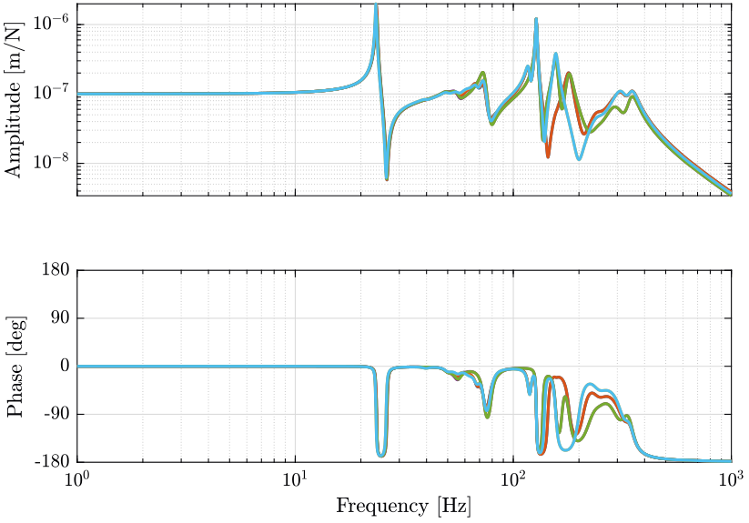
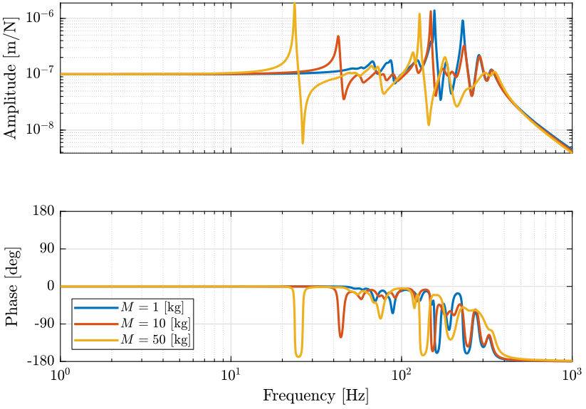
Let’s look at the transfer function from actuator forces in the nano-hexapod to the measured displacement of the actuator for all 6 pairs of actuator/sensor (figure 35).

Figure 35: Transfer function from forces applied in the legs to leg displacement sensor (png, pdf)

4.1.2 Control Design

The Direct Velocity Feedback is defined below. A Low pass Filter is added to make the controller transfer function proper.

K_dvf = s*30000/(1 + s/2/pi/10000);

The obtained loop gains are shown in figure 36.

Figure 36: Loop Gain for the Integral Force Feedback (png, pdf)

4.1.3 Diagonal Controller

We create the diagonal controller and we add a minus sign as we have a positive feedback architecture.

K_dvf = -K_dvf*eye(6);

We save the controller for further analysis.

save('./mat/active_damping_K_dvf.mat', 'K_dvf');

4.2 Tomography Experiment

4.2.1 Initialize the Simulation

We initialize elements for the tomography experiment.

prepareTomographyExperiment();

We set the DVF controller.

load('./mat/active_damping_K_dvf.mat', 'K_dvf');
initializeController('type', 'dvf');

We change the simulation stop time.

load('mat/conf_simulink.mat');
set_param(conf_simulink, 'StopTime', '4.5');

And we simulate the system.

sim('nass_model');

Finally, we save the simulation results for further analysis

En_dvf = En;
Eg_dvf = Eg;
save('./mat/active_damping_tomo_exp.mat', 'En_dvf', 'Eg_dvf', '-append');

4.2.2 Compare with Undamped system

Figure 37: Position Error during tomography experiment - XY Motion (png, pdf)

Figure 38: Position Error during tomography experiment - Translations (png, pdf)

Figure 39: Position Error during tomography experiment - Rotations (png, pdf)

4.3 Conclusion

Direct Velocity Feedback using a relative motion sensor:

Robust (guaranteed stability)

5 Inertial Control

All the files (data and Matlab scripts) are accessible here.

In Inertial Control, a feedback is applied between the measured absolute motion (velocity or acceleration) of the platform to the actuator force input.

5.1 Control Design

5.1.1 Plant

Let’s load the undamped plant:

load('./mat/active_damping_undamped_plants.mat', 'G_ine');
load('./mat/active_damping_plants_variable.mat', 'masses', 'Gm_ine');

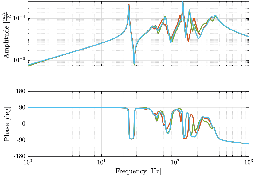
Let’s look at the transfer function from actuator forces in the nano-hexapod to the measured velocity of the nano-hexapod platform in the direction of the corresponding actuator for all 6 pairs of actuator/sensor (figure 40).

Figure 40: Transfer function from forces applied in the legs to leg velocity sensor (png, pdf)

5.1.2 Control Design

The controller is defined below and the obtained loop gain is shown in figure 41.

K_ine = 2.5e4;

Figure 41: Loop Gain for Inertial Control (png, pdf)

5.1.3 Diagonal Controller

We create the diagonal controller and we add a minus sign as we have a positive feedback architecture.

K_ine = -K_ine*eye(6);

We save the controller for further analysis.

save('./mat/active_damping_K_ine.mat', 'K_ine');

5.2 Conclusion

Inertial Control should not be used.

6 Comparison

6.1 Load the plants

load('./mat/active_damping_plants.mat', 'G', 'G_iff', 'G_ine', 'G_dvf');

6.2 Sensitivity to Disturbance

Figure 42: Sensitivity to ground motion in the Z direction on the Z motion error (png, pdf)

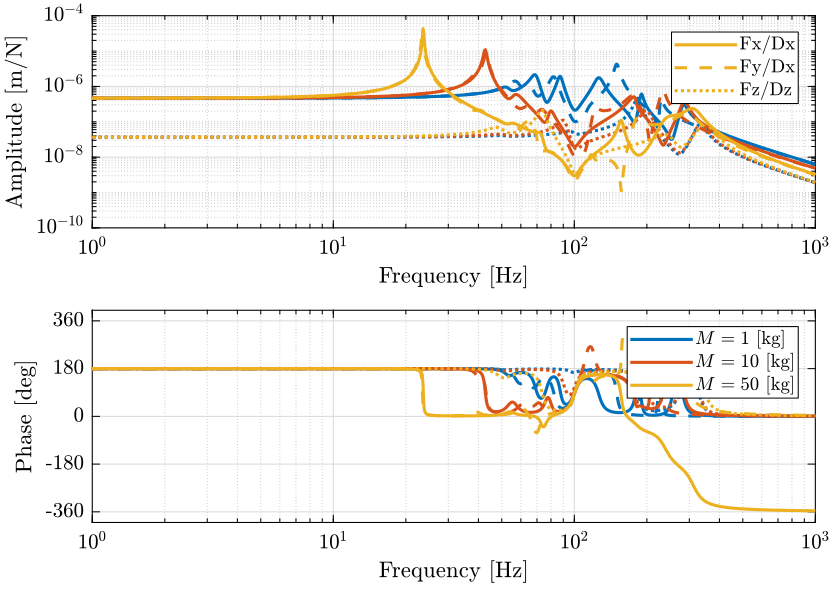
Figure 43: Compliance in the Z direction: Sensitivity of direct forces applied on the sample in the Z direction on the Z motion error (png, pdf)

Figure 44: Sensitivity to forces applied in the Z direction by the Spindle on the Z motion error (png, pdf)

Figure 45: Sensitivity to forces applied in the Z direction by the Y translation stage on the Z motion error (png, pdf)

Figure 46: Sensitivity to forces applied in the X direction by the Y translation stage on the X motion error (png, pdf)

6.3 Damped Plant

Figure 47: Plant for the \(z\) direction for different active damping technique used (png, pdf)

Figure 48: Plant for the \(x\) direction for different active damping technique used (png, pdf)

Figure 49: Comparison of one off-diagonal plant for different damping technique applied (png, pdf)

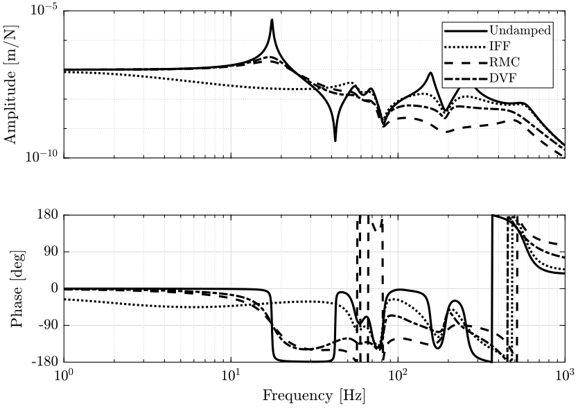
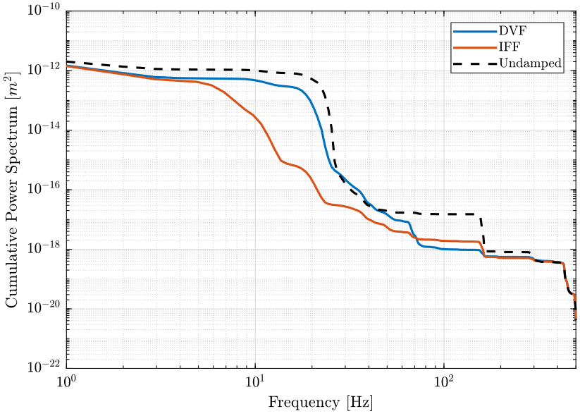
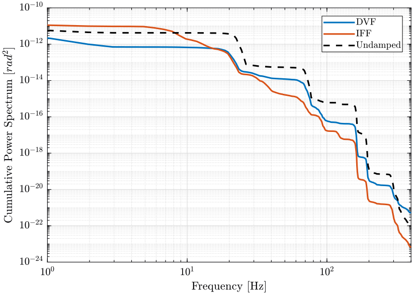
6.4 Tomography Experiment - Frequency Domain analysis

load('./mat/active_damping_tomo_exp.mat', 'En', 'En_iff', 'En_dvf');
Fs = 1e3; % Sampling Frequency of the Data
t = (1/Fs)*[0:length(En(:,1))-1];

We remove the first 0.5 seconds where the transient behavior is fading out.

[~, i_start] = min(abs(t - 0.5)); % find the indice corresponding to 0.5s

t = t(i_start:end) - t(i_start);
En = En(i_start:end, :);
En_dvf = En_dvf(i_start:end, :);
En_iff = En_iff(i_start:end, :);

Window used for pwelch function.

n_av = 4;
han_win = hanning(ceil(length(En(:, 1))/n_av));

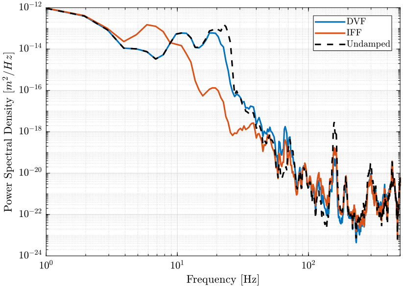
Figure 50: PSD of the translation errors in the X direction for applied Active Damping techniques (png, pdf)

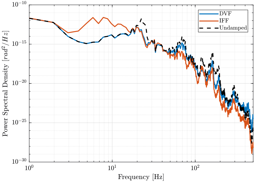
Figure 51: PSD of the rotation errors in the X direction for applied Active Damping techniques (png, pdf)

Figure 52: CPS of the translation errors in the X direction for applied Active Damping techniques (png, pdf)

Figure 53: CPS of the rotation errors in the X direction for applied Active Damping techniques (png, pdf)

7 Useful Functions

7.1 prepareLinearizeIdentification

This Matlab function is accessible here.

Function Description

function [] = prepareLinearizeIdentification(args)

Optional Parameters

arguments
    args.nass_actuator       char   {mustBeMember(args.nass_actuator,{'piezo', 'lorentz'})} = 'piezo'
    args.sample_mass   (1,1) double {mustBeNumeric, mustBePositive} = 50 % [kg]
end

Initialize the Simulation

We initialize all the stages with the default parameters.

initializeGround();
initializeGranite();
initializeTy();
initializeRy();
initializeRz();
initializeMicroHexapod();
initializeAxisc();
initializeMirror();

The nano-hexapod is a piezoelectric hexapod and the sample has a mass of 50kg.

initializeNanoHexapod('actuator', args.nass_actuator);
initializeSample('mass', args.sample_mass);

We set the references and disturbances to zero.

initializeReferences();
initializeDisturbances('enable', false);

We set the controller type to Open-Loop.

initializeController('type', 'open-loop');

And we put some gravity.

initializeSimscapeConfiguration('gravity', true);

We do not need to log any signal.

initializeLoggingConfiguration('log', 'none');

7.2 prepareTomographyExperiment

This Matlab function is accessible here.

Function Description

function [] = prepareTomographyExperiment(args)

Optional Parameters

arguments
    args.nass_actuator       char   {mustBeMember(args.nass_actuator,{'piezo', 'lorentz'})} = 'piezo'
    args.sample_mass   (1,1) double {mustBeNumeric, mustBePositive} = 50 % [kg]
    args.Rz_period     (1,1) double {mustBeNumeric, mustBePositive} = 1 % [s]
end

Initialize the Simulation

We initialize all the stages with the default parameters.

initializeGround();
initializeGranite();
initializeTy();
initializeRy();
initializeRz();
initializeMicroHexapod();
initializeAxisc();
initializeMirror();

The nano-hexapod is a piezoelectric hexapod and the sample has a mass of 50kg.

initializeNanoHexapod('actuator', args.nass_actuator);
initializeSample('mass', args.sample_mass);

We set the references that corresponds to a tomography experiment.

initializeReferences('Rz_type', 'rotating', 'Rz_period', args.Rz_period);

initializeDisturbances();

Open Loop.

initializeController('type', 'open-loop');

And we put some gravity.

initializeSimscapeConfiguration('gravity', true);

We log the signals.

initializeLoggingConfiguration('log', 'all');

Active Damping applied on the Simscape Model

Table of Contents

1 Undamped System

1.1 Identification of the dynamics for Active Damping

1.1.1 Identification

1.1.2 Obtained Plants for Active Damping

1.2 Identification of the dynamics for High Authority Control

1.2.1 Identification

1.2.2 Obtained Plants

1.3 Tomography Experiment

1.3.1 Simulation

1.3.2 Results

2 Variability of the system dynamics for Active Damping

2.1 Variation of the Sample Mass

2.2 Variation of the Spindle Angle

2.3 Variation of the Spindle Rotation Speed

2.3.1 Dynamics of the Active Damping plants

2.3.2 Variation of the poles and zeros with the Spindle rotation frequency

2.4 Variation of the Tilt Angle

2.5 Scans of the Translation Stage

2.6 Conclusion

3 Integral Force Feedback

3.1 Control Design

3.1.1 Plant

3.1.2 Control Design

3.1.3 Diagonal Controller

3.2 Tomography Experiment

3.2.1 Simulation with IFF Controller

3.2.2 Compare with Undamped system

3.3 Conclusion

4 Direct Velocity Feedback

4.1 Control Design

4.1.1 Plant

4.1.2 Control Design

4.1.3 Diagonal Controller

4.2 Tomography Experiment

4.2.1 Initialize the Simulation

4.2.2 Compare with Undamped system

4.3 Conclusion

5 Inertial Control

5.1 Control Design

5.1.1 Plant

5.1.2 Control Design

5.1.3 Diagonal Controller

5.2 Conclusion

6 Comparison

6.1 Load the plants

6.2 Sensitivity to Disturbance

6.3 Damped Plant

6.4 Tomography Experiment - Frequency Domain analysis

7 Useful Functions

7.1 prepareLinearizeIdentification

Function Description

Optional Parameters

Initialize the Simulation

7.2 prepareTomographyExperiment

Function Description

Optional Parameters

Initialize the Simulation