Design of the Nano-Hexapod and associated Control Architectures - Summary
Table of Contents
- 1. Feedback Systems and Noise budgeting
- 2. Identification of the Micro-Station Dynamics
- 3. Identification of the Disturbances
- 4. Multi Body Model
- 5. Optimal Nano-Hexapod Design
- 6. Robust Control Architecture
The overall objective is to design a nano-hexapod an the associated control architecture that allows the stabilization of samples down to \(\approx 10nm\) in presence of disturbances and system variability.
To understand the design challenges of such system, a short introduction to Feedback control is provided in Section 1. The mathematical tools (Power Spectral Density, Noise Budgeting, …) that will be used throughout this study are also introduced.
To be able to develop both the nano-hexapod and the control architecture in an optimal way, we need a good estimation of:
- the micro-station dynamics (Section 2)
- the frequency content of the important source of disturbances in play such as vibration of stages and ground motion (Section 3)
We then develop a model of the system that must represent all the important physical effects in play. Such model is presented in Section 4.
A modular model of the nano-hexapod is then included in the system. The effects of the nano-hexapod characteristics on the dynamics are then studied. Based on that, an optimal choice of the nano-hexapod stiffness is made (Section 5).
Finally, using the optimally designed nano-hexapod, a robust control architecture is developed. Simulations are performed to show that this design gives acceptable performance and the required robustness (Section 6).
1 Feedback Systems and Noise budgeting
1.1 Simple Feedback System
We usually analyze dynamical systems in the frequency domain using the Laplace transform.
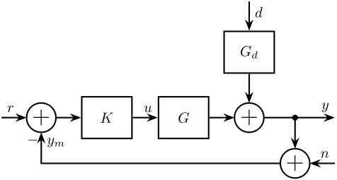
Figure 1: Figure caption
- \(y\) is the relative position of the sample with respect to the granite
- \(d\) is the disturbances affecting \(y\) (ground motion, vibration of stages)
- \(n\) is the noise of the sensor measuring \(y\)
- \(r\) is the reference signal, corresponding to the wanted \(y\)
- we note \(\epsilon = r - y\) the position error
\[ \epsilon = \frac{1}{1 + GK} r + \frac{GK}{1 + GK} n - \frac{G_d}{1 + GK} d \]
We usually note:
\begin{align} S &= \frac{1}{1 + GK} \\ T &= \frac{GK}{1 + GK} \end{align}\(S\) is called the sensibility transfer function and \(T\) the transmissibility transfer function.
And we have: \[ \epsilon = S r + T n - G_d S d \]
Thus, we usually want \(|S|\) small such that the effect of disturbances are reduced down to acceptable levels and such that the system is able to follow the change of reference with only small tracking errors.
However, when \(|S|\) is small, \(|T| \approx 1\) and all the sensor noise is transmitted to the position error.
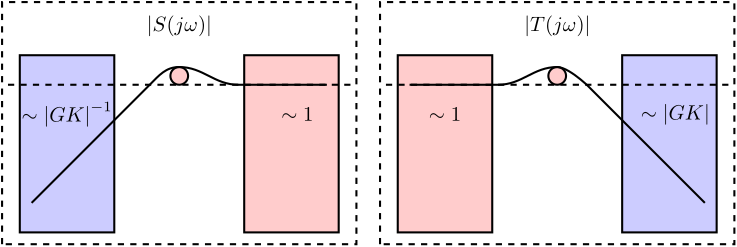
Figure 2: Figure caption
The nano-hexapod characteristics will change both \(G\) and \(G_d\).
1.2 Noise Budgeting
1.2.1 Power Spectral Density
The Power Spectral Density (PSD) \(S_{xx}(f)\) of the time domain \(x(t)\) (in \([m]\)) can be computed using the following equation: \[ S_{xx}(f) = \frac{1}{f_s} \sum_{m=-\infty}^{\infty} R_{xx}(m) e^{-j 2 \pi m f / f_s} \ \left[\frac{m^2}{\text{Hz}}\right] \] where
- \(f_s\) is the sampling frequency in \([Hz]\)
- \(R_{xx}\) is the autocorrelation
The PSD \(S_{xx}(f)\) represents the distribution of the (average) signal power over frequency.
Thus, the total power in the signal can be obtained by integrating these infinitesimal contributions, the Root Mean Square (RMS) value of the signal \(x(t)\) is then:
\begin{equation} x_{\text{rms}} = \sqrt{\int_{0}^{\infty} S_{xx}(f) df} \ [m,\text{rms}] \end{equation}One can also integrate the infinitesimal power \(S_{xx}(f)df\) over a finite frequency band to obtain the power of the signal \(x\) in that frequency band:
\begin{equation} P_{f_1,f_2} = \int_{f_1}^{f_2} S_{xx}(f) df \quad [m^2] \end{equation}1.2.2 Cumulative Power Spectrum
The Cumulative Power Spectrum is the cumulative integral of the Power Spectral Density starting from \(0\ \text{Hz}\) with increasing frequency:
\begin{equation} CPS_x(f) = \int_0^f S_{xx}(\nu) d\nu \quad [\text{unit}^2] \end{equation}The Cumulative Power Spectrum taken at frequency \(f\) thus represent the power in the signal in the frequency band \(0\) to \(f\).
An alternative definition of the Cumulative Power Spectrum can be used where the PSD is integrated from \(f\) to \(\infty\):
\begin{equation} CPS_x(f) = \int_f^\infty S_{xx}(\nu) d\nu \quad [\text{unit}^2] \end{equation}And thus \(CPS_x(f)\) represents the power in the signal \(x\) for frequencies above \(f\).
The Cumulative Power Spectrum can be used to determine in which frequency band the effect of disturbances should be reduced and the approximated required control bandwidth in order to obtained some specified vibration amplitude.
1.2.3 Modification of a signal’s PSD when going through an LTI system
Let’s consider a signal \(u\) with a PSD \(S_{uu}\) going through a LTI system \(G(s)\) that outputs a signal \(y\) with a PSD (Figure 3).

The Power Spectral Density of the output signal \(y\) can be computed using:
\begin{equation} S_{yy}(\omega) = \left|G(j\omega)\right|^2 S_{uu}(\omega) \end{equation}1.2.4 PSD of combined signals
Let’s consider a signal \(y\) that is the sum of two uncorrelated signals \(u\) and \(v\).
We have that the PSD of \(y\) is equal to sum of the PSD and \(u\) and the PSD of \(v\): \[ S_{yy} = S_{uu} + S_{vv} \]

1.2.5 Dynamic Noise Budgeting
Let’s consider the Feedback architecture,
The position error \(\epsilon\) is equal to: \[ \epsilon = S r + T n - G_d S d \]
If we suppose that the signals \(r\), \(n\) and \(d\) are uncorrelated, the PSD of \(\epsilon\) is: \[ S_{\epsilon \epsilon}(\omega) = |S(j\omega)|^2 S_{rr}(\omega) + |T(j\omega)|^2 S_{nn}(\omega) + |G_d(j\omega) S(j\omega)|^2 S_{dd}(\omega) \]
And the RMS residual motion is equal to:
\begin{align*} \epsilon_\text{rms} &= \sqrt{ \int_0^\infty S_{\epsilon\epsilon}(\omega) d\omega} \\ &= \sqrt{ \int_0^\infty |S(j\omega)|^2 S_{rr}(\omega) + |T(j\omega)|^2 S_{nn}(\omega) + |G_d(j\omega) S(j\omega)|^2 S_{dd}(\omega) d\omega } \end{align*}To estimate the PSD of the position error \(\epsilon\) and thus the RMS residual motion, we need:
- The Power Spectral Densities of the signals affecting the system:
- \(S_{rr}\)
- \(S_{nn}\)
- \(S_{dd}\)
- The dynamics of the system \(G\), \(G_d\) and the controller \(K\) (or alternatively \(S\), \(T\) and \(G_d\))
1.3 Trade off Robustness / Performance
If we want high level of performance, the experimental conditions should be carefully controlled.
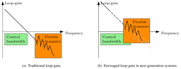
Figure 5: Envisaged developments in motion systems. In traditional motion systems, the control bandwidth takes place in the rigid-body region. In the next generation systemes, flexible dynamics are foreseen to occur within the control bandwidth. oomen18_advan_motion_contr_precis_mechat
Limitation of feedback control:
- bandwidth is limited at a frequency where the behavior of the system is not known
Predictible system.
For instance, ASML, everything is calibrated (wafer, some size, mass, etc…)
Here, the main difficulty is that we want a very high performance system that is robust to change of:
- Micro Station Configuration: position of the stages, change of on stage
- Payload mass and dynamics
- Spindle’s rotation speed
1.4 Sensibility Transfer Function and Control Bandwidth
When applying feedback in a system, it is much more convenient to look at things in the frequency domain.
[ ]Add a
we will generally decrease the effect of the disturbances
[ ]Find the citation where it is said that the bandwidth is the consequence of the wanted disturbance rejection at some lower frequency
2 Identification of the Micro-Station Dynamics
https://tdehaeze.github.io/meas-analysis/
Modal Analysis: https://tdehaeze.github.io/meas-analysis/modal-analysis/index.html
The obtained dynamics will allows us to compare the dynamics of the model.
2.1 Setup
In order to perform to Modal Analysis and to obtain first a response model, the following devices were used:
- An acquisition system (OROS) with 24bits ADCs
- 3 tri-axis Accelerometers
- An Instrumented Hammer
The measurement thus consists of:
- Exciting the structure at the same location with the Hammer (Figure 7)
- Move the accelerometers to measure all the DOF of the structure.
The position of the accelerometers are:
- 4 on the first granite
- 4 on the second granite
- 4 on top of the translation stage (figure 6)
- 4 on top of the tilt stage
- 3 on top of the spindle
- 4 on top of the hexapod
In total, 69 degrees of freedom are measured (23 tri axis accelerometers).
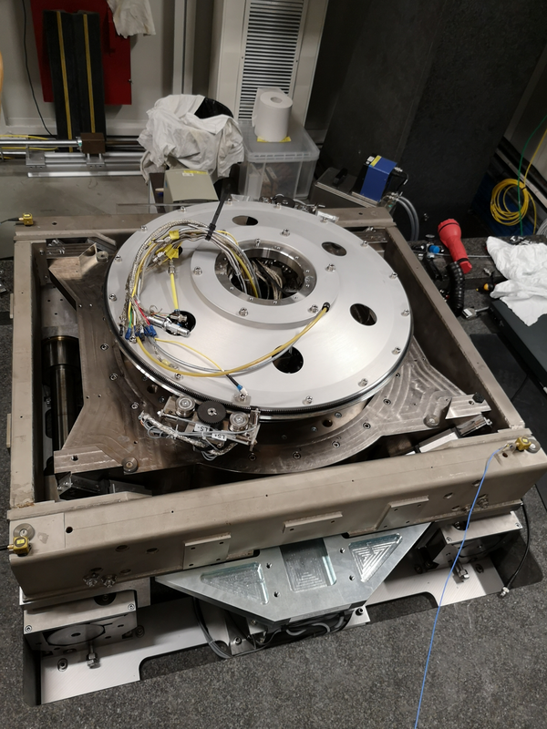
Figure 6: Figure caption
Figure 7: Figure caption
2.2 Results
From the measurements, we obtain
- Reduction of the
- solid body assumption
- verification of the assumption => ok
Figure 8: Figure caption
Figure 9: Figure caption
2.3 Conclusion
The reduction of the number of degrees of freedom from 69 (23 accelerometers with each 3DOF) to 36 (6 solid bodies with 6 DOF) seems to work well.
This confirms the fact that the stages are indeed behaving as a solid body in the frequency band of interest. This valid the fact that a multi-body model can be used to represent the dynamics of the micro-station.
3 Identification of the Disturbances
https://tdehaeze.github.io/meas-analysis/
Open Loop Noise budget: https://tdehaeze.github.io/nass-simscape/disturbances.html
Static Guiding errors:
- measured at the PEL
- low frequency errors, will thus be compensated
The problem are on the high frequency disturbances
3.2 Stage Vibration - Effect of Control systems
Control system of each stage has been tested https://tdehaeze.github.io/meas-analysis/disturbance-control-system/index.html https://tdehaeze.github.io/meas-analysis/2018-10-15%20-%20Marc/index.html
25Hz vertical motion when the Spindle is turned on (even when not rotating).
3.3 Stage Vibration - Effect of Motion
3.4 Sum of all disturbances
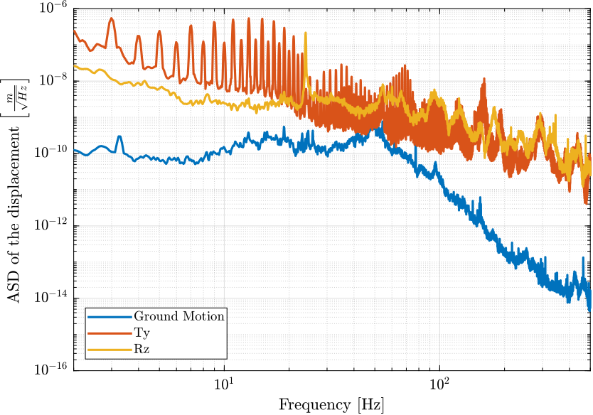
Figure 10: Amplitude Spectral Density fo the motion error due to disturbances
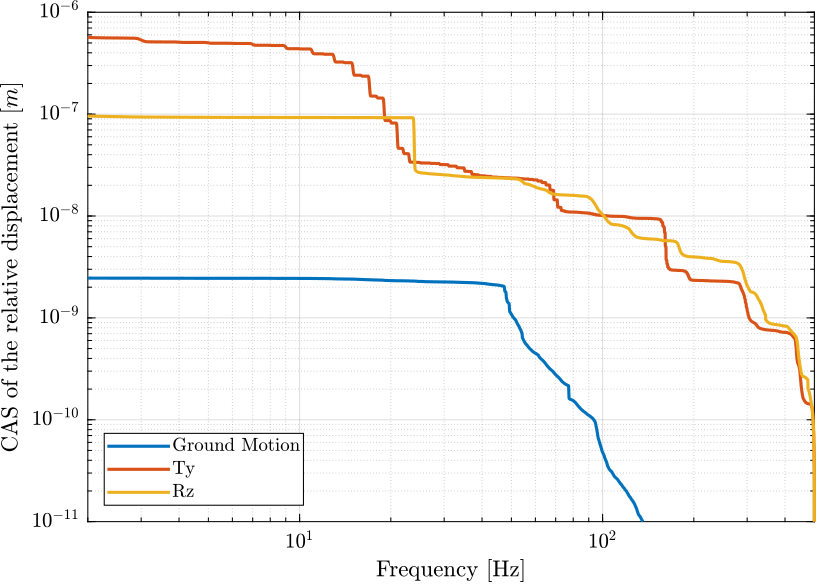
Figure 11: Cumulative Amplitude Spectrum of the motion error due to disturbances
Expected required bandwidth
3.5 Better measurement of the effect of disturbances
Here, the measurement were made with inertial sensors. However, we are interested in the relative motion of the sample with respect to the granite and not the absolute motion.
The best measurement of the disturbances would be to have the metrology already functioning.
We could perform a measurement using the X-ray.
Detector Requirement:
- Sample frequency above \(400Hz\)
- Resolution of \(\approx 20nm\)
3.6 Conclusion
4 Multi Body Model
4.1 Validity of the model
The mass/inertia of each stage is automatically computed from the geometry and the density of the materials.
The stiffness of each joint is first set to measured values or stiffness from data sheets.
Then, the values of the stiffness and damping of each joint is manually tuned until the obtained dynamics is sufficiently close to the measured dynamics.
We could, from the measurement, automatically extract the stiffness and damping values, we this would have required a lot of work and having a perfect match is not required here.
Comparison model - measurements : https://tdehaeze.github.io/nass-simscape/identification.html
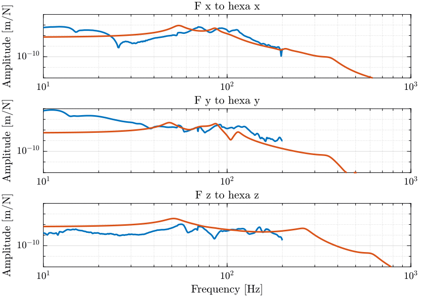
Figure 12: Figure caption
4.2 Wanted position of the sample and position error
From the reference position of each stage, we can compute the wanted pose of the sample with respect to the granite. This is done with multiple transformation matrices.
Then, from the measurement of the metrology corresponding to the position of the sample with respect to the granite, we can compute the position error of the sample expressed in a frame fixed to the nano-hexapod.
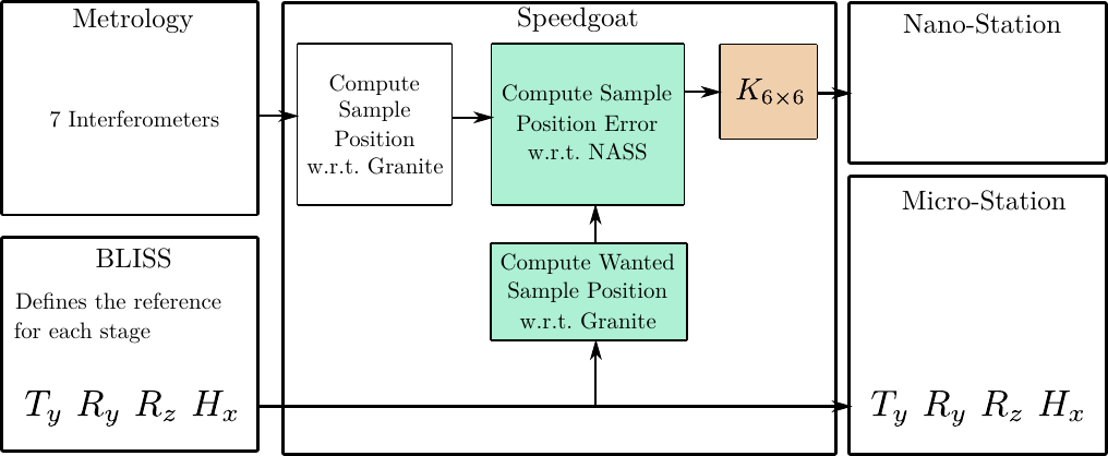
Figure 13: Figure caption
Measurement of the sample’s position - conversion of positioning error in the frame of the Nano-hexapod for control: https://tdehaeze.github.io/nass-simscape/positioning_error.html
4.3 Simulation of Experiments
Now that the
- dynamics of the model is tuned
- disturbances are included in the model
We can perform simulation of experiments.
https://tdehaeze.github.io/nass-simscape/experiments.html
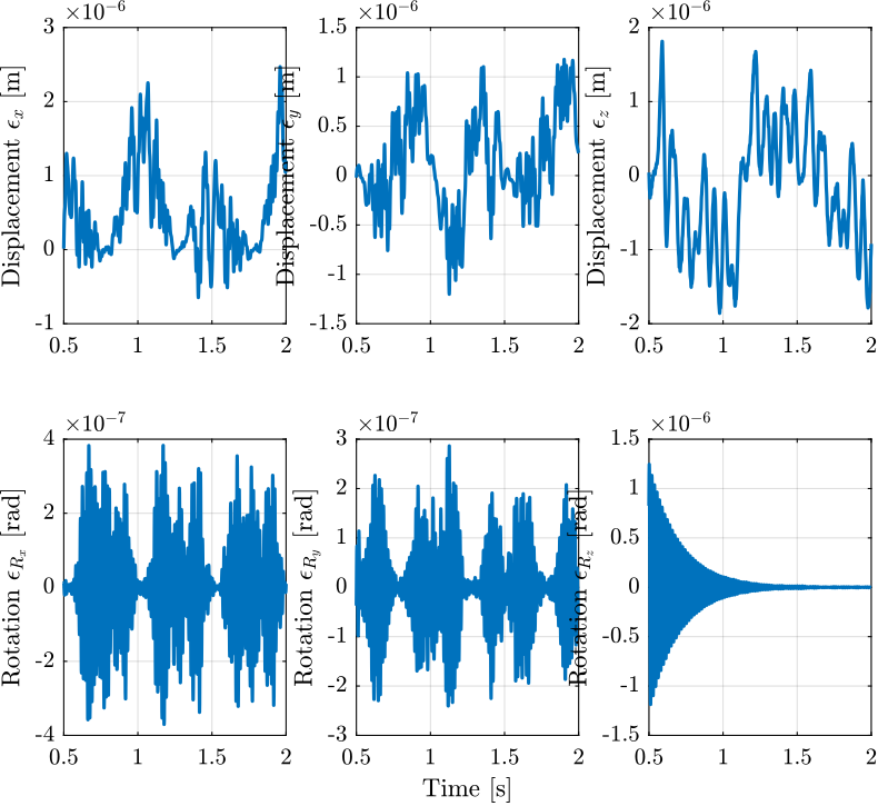
Figure 14: Position error of the Sample with respect to the granite during a Tomography Experiment with included disturbances
4.4 Conclusion
Possible to study many effects. Extraction of transfer function like \(G\) and \(G_d\).
Simulation of experiments to validate performance.
5 Optimal Nano-Hexapod Design
As explain before, the nano-hexapod properties (mass, stiffness, architecture, …) will influence:
- the plant dynamics \(G\)
- the effect of disturbances \(G_d\)
We which here to choose the nano-hexapod properties such that:
- has an easy
- minimize the
- minimize \(|G_d|\)
5.1 Optimal Stiffness to reduce the effect of disturbances
5.2 Optimal Stiffness
The goal is to design a system that is robust.
Thus, we have to identify the sources of uncertainty and try to minimize them.
Uncertainty in the system can be caused by:
- Effect of Support Compliance: https://tdehaeze.github.io/nass-simscape/uncertainty_support.html
- Effect of Payload Dynamics: https://tdehaeze.github.io/nass-simscape/uncertainty_payload.html
- Effect of experimental condition (micro-station pose, spindle rotation): https://tdehaeze.github.io/nass-simscape/uncertainty_experiment.html
All these uncertainty will limit the maximum attainable bandwidth.
Fortunately, the nano-hexapod stiffness have an influence on the dynamical uncertainty induced by the above effects.
Determination of the optimal stiffness based on all the effects:
The main performance limitation are payload variability
Main problem: heavy samples with small stiffness. The first resonance frequency of the sample will limit the performance.
The nano-hexapod stiffness will also change the sensibility to disturbances.
Effect of Nano-hexapod stiffness on the Sensibility to disturbances: https://tdehaeze.github.io/nass-simscape/optimal_stiffness_disturbances.html
5.3 Sensors to be included
Ways to damp:
- Force Sensor
- Relative Velocity Sensors
- Inertial Sensor
https://tdehaeze.github.io/rotating-frame/index.html
Sensors to be included: