Design of the Nano-Hexapod and associated Control Architectures - Summary

1. Introduction to Feedback Systems and Noise budgeting
- 1.1. Feedback System
- 1.2. Dynamic error budgeting
2. Identification of the Micro-Station Dynamics
3. Identification of the Disturbances
4. Multi Body Model
5. Optimal Nano-Hexapod Design
6. Robust Control Architecture
7. Further notes

The overall objective is to design a nano-hexapod an the associated control architecture that allows the stabilization of samples down to \(\approx 10nm\) in presence of disturbances and system variability.

To understand the design challenges of such system, a short introduction to Feedback control is provided in Section 1. The mathematical tools (Power Spectral Density, Noise Budgeting, …) that will be used throughout this study are also introduced.

To be able to develop both the nano-hexapod and the control architecture in an optimal way, we need a good estimation of:

the micro-station dynamics (Section 2)
the frequency content of the important source of disturbances in play such as vibration of stages and ground motion (Section 3)

We then develop a model of the system that must represent all the important physical effects in play. Such model is presented in Section 4.

A modular model of the nano-hexapod is then included in the system. The effects of the nano-hexapod characteristics on the dynamics are then studied. Based on that, an optimal choice of the nano-hexapod stiffness is made (Section 5).

Finally, using the optimally designed nano-hexapod, a robust control architecture is developed. Simulations are performed to show that this design gives acceptable performance and the required robustness (Section 6).

1 Introduction to Feedback Systems and Noise budgeting

In this section, we first introduce some basics of feedback systems (Section 1.1). This should highlight the challenges in terms of combined performance and robustness.

In Section 1.2 is introduced the dynamic error budgeting which is a powerful tool that allows to derive the total error in a dynamic system from multiple disturbance sources. This tool will be widely used throughout this study to both predict the performances and identify the effects that do limit the performances.

1.1 Feedback System

The use of feedback control as several advantages and pitfalls that are listed below (taken from schmidt14_desig_high_perfor_mechat_revis_edition):

Advantages:
- Reduction of the effect of disturbances: Disturbances affecting the sample vibrations are observed by the sensor signal, and therefore the feedback controller can compensate for them
- Handling of uncertainties: Feedback controlled systems can also be designed for robustness, which means that the stability and performance requirements are guaranteed even for parameter variation of the controller mechatronics system
Pitfalls:
- Limited reaction speed: A feedback controller reacts on the difference between the reference signal (wanted motion) and the measurement (actual motion), which means that the error has to occur first before the controller can correct for it. The limited reaction speed means that the controller will be able to compensate the positioning errors only in some frequency band, called the controller bandwidth
- Feedback of noise: By closing the loop, the sensor noise is also fed back and will induce positioning errors
- Can introduce instability: Feedback control can destabilize a stable plant. Thus the robustness properties of the feedback system must be carefully guaranteed

1.1.1 Simplified Feedback Control Diagram for the NASS

Let’s consider the block diagram shown in Figure 1 where the signals are:

\(y\): the relative position of the sample with respect to the granite (the quantity we wish to control)
\(d\): the disturbances affecting \(y\) (ground motion, vibration of stages)
\(n\): the noise of the sensor measuring \(y\)
\(r\): the reference signal, corresponding to the wanted \(y\)
\(\epsilon = r - y\): the position error

And the dynamical blocks are:

\(G\): representing the dynamics from forces/torques applied by the nano-hexapod to the relative position sample/granite \(y\)
\(G_d\): representing how the disturbances (e.g. ground motion) are affecting the relative position sample/granite \(y\)
\(K\): representing the controller (to be designed)

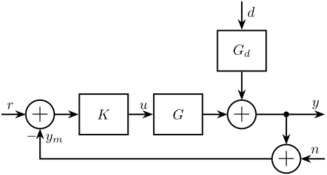
Figure 1: Block Diagram of a simple feedback system

Without the use of feedback (i.e. nano-hexapod), the disturbances will induce a sample motion error equal to:

\begin{equation} y = G_d d \label{eq:open_loop_error} \end{equation}

which is out of the specifications (micro-meter range compare to the required \(\approx 10nm\)).

In the next section, we see how the use of the feedback system permits to lower the effect of the disturbances \(d\) on the sample motion error.

1.1.2 How does the feedback loop is modifying the system behavior?

If we write down the position error signal \(\epsilon = r - y\) as a function of the reference signal \(r\), the disturbances \(d\) and the measurement noise \(n\) (using the feedback diagram in Figure 1), we obtain: \[ \epsilon = \frac{1}{1 + GK} r + \frac{GK}{1 + GK} n - \frac{G_d}{1 + GK} d \]

We usually note:

\begin{align} S &= \frac{1}{1 + GK} \\ T &= \frac{GK}{1 + GK} \end{align}

where \(S\) is called the sensibility transfer function and \(T\) the transmissibility transfer function.

And the position error can be rewritten as:

\begin{equation} \epsilon = S r + T n - G_d S d \label{eq:closed_loop_error} \end{equation}

From Eq. \eqref{eq:closed_loop_error} representing the closed-loop system behavior, we can see that:

the effect of disturbances \(d\) on \(\epsilon\) is multiplied by a factor \(S\) compared to the open-loop case
the measurement noise \(n\) is injected and multiplied by a factor \(T\)

Ideally, we would like to design the controller \(K\) such that:

\(|S|\) is small to limit the effect of disturbances
\(|T|\) is small to limit the injection of sensor noise

As shown in the next section, there is a trade-off between the disturbance reduction and the noise injection.

1.1.3 Trade off: Disturbance Reduction / Noise Injection

We have from the definition of \(S\) and \(T\) that:

\begin{equation} S + T = \frac{1}{1 + GK} + \frac{GK}{1 + GK} = 1 \end{equation}

meaning that we cannot have \(|S|\) and \(|T|\) small at the same time.

There is therefore a trade-off between the disturbance rejection and the measurement noise filtering.

Typical shapes of \(|S|\) and \(|T|\) as a function of frequency are shown in Figure 2. We can observe that \(|S|\) and \(|T|\) exhibit different behaviors depending on the frequency band:

At low frequency (inside the control bandwidth):
- \(|S|\) can be made small and thus the effect of disturbances is reduced
- \(|T| \approx 1\) and all the sensor noise is transmitted
At high frequency (outside the control bandwidth):
- \(|S| \approx 1\) and the feedback system does not reduce the effect of disturbances
- \(|T|\) is small and thus the sensor noise is filtered
Near the crossover frequency (between the two frequency bands):
- The effect of disturbances is increased

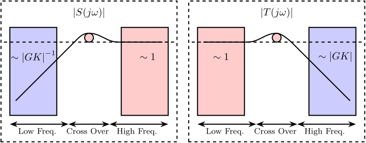
Figure 2: Typical shapes and constrain of the Sensibility and Transmibility closed-loop transfer functions

1.1.4 Trade off: Robustness / Performance

As shown in the previous section, the effect of disturbances is reduced inside the control bandwidth.

Moreover, the slope of \(|S(j\omega)|\) is limited for stability reasons (not explained here), and therefore a large control bandwidth is required to obtain sufficient disturbance rejection at lower frequencies (where the disturbances have large effects).

The next important question is what effects do limit the attainable control bandwidth?

The main issue it that for stability reasons, the behavior of the mechanical system must be known with only small uncertainty in the vicinity of the crossover frequency.

For mechanical systems, this generally means that control bandwidth should take place before any appearing of flexible dynamics (Right part of Figure 3).

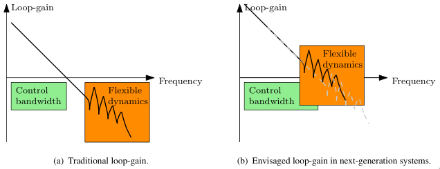
Figure 3: Envisaged developments in motion systems. In traditional motion systems, the control bandwidth takes place in the rigid-body region. In the next generation systemes, flexible dynamics are foreseen to occur within the control bandwidth. oomen18_advan_motion_contr_precis_mechat

This also means that any possible change in the system should have a small impact on the system dynamics in the vicinity of the crossover.

For the NASS, the possible changes in the system are:

a modification of the payload mass and dynamics
a change of experimental condition: spindle’s rotation speed, position of each micro-station’s stage
a change in the micro-station dynamics (change of mechanical elements, aging effect, …)

The nano-hexapod and the control architecture have to be developed such that the feedback system remains stable and exhibit acceptable performance for all these possible changes in the system.

This problem of robustness represent one of the main challenge for the design of the NASS.

1.2 Dynamic error budgeting

The dynamic error budgeting is a powerful tool to study the effect of multiple error sources and to see how the feedback system does reduce the effect

To understand how to use and understand it, the Power Spectral Density and the Cumulative Power Spectrum are first introduced. Then, is shown how does multiple error sources are combined and modified by dynamical systems.

Finally,

1.2.1 Power Spectral Density

The Power Spectral Density (PSD) \(S_{xx}(f)\) of the time domain signal \(x(t)\) is defined as the Fourier transform of the autocorrelation function: \[ S_{xx}(\omega) = \int_{-\infty}^{\infty} R_{xx}(\tau) e^{-j \omega \tau} d\tau \ \frac{[\text{unit of } x]^2}{\text{Hz}} \]

The PSD \(S_{xx}(\omega)\) represents the distribution of the (average) signal power over frequency.

Thus, the total power in the signal can be obtained by integrating these infinitesimal contributions, the Root Mean Square (RMS) value of the signal \(x(t)\) is then:

\begin{equation} x_{\text{rms}} = \sqrt{\int_{0}^{\infty} S_{xx}(\omega) d\omega} \end{equation}

One can also integrate the infinitesimal power \(S_{xx}(\omega)d\omega\) over a finite frequency band to obtain the power of the signal \(x\) in that frequency band:

\begin{equation} P_{f_1,f_2} = \int_{f_1}^{f_2} S_{xx}(\omega) d\omega \quad [\text{unit of } x]^2 \end{equation}

1.2.2 Cumulative Power Spectrum

The Cumulative Power Spectrum is the cumulative integral of the Power Spectral Density starting from \(0\ \text{Hz}\) with increasing frequency:

\begin{equation} CPS_x(f) = \int_0^f S_{xx}(\nu) d\nu \quad [\text{unit of } x]^2 \end{equation}

The Cumulative Power Spectrum taken at frequency \(f\) thus represent the power in the signal in the frequency band \(0\) to \(f\).

An alternative definition of the Cumulative Power Spectrum can be used where the PSD is integrated from \(f\) to \(\infty\):

\begin{equation} CPS_x(f) = \int_f^\infty S_{xx}(\nu) d\nu \quad [\text{unit of } x]^2 \end{equation}

And thus \(CPS_x(f)\) represents the power in the signal \(x\) for frequencies above \(f\).

The Cumulative Power Spectrum will be used to determine in which frequency band the effect of disturbances should be reduced, and thus the approximate required control bandwidth.

1.2.3 Modification of a signal’s PSD when going through an LTI system

Let’s consider a signal \(u\) with a PSD \(S_{uu}\) going through a LTI system \(G(s)\) that outputs a signal \(y\) with a PSD (Figure 4).

Figure 4: LTI dynamical system \(G(s)\) with input signal \(u\) and output signal \(y\)

The Power Spectral Density of the output signal \(y\) can be computed using:

\begin{equation} S_{yy}(\omega) = \left|G(j\omega)\right|^2 S_{uu}(\omega) \end{equation}

1.2.4 PSD of combined signals

Let’s consider a signal \(y\) that is the sum of two uncorrelated signals \(u\) and \(v\) (Figure 5).

We have that the PSD of \(y\) is equal to sum of the PSD and \(u\) and the PSD of \(v\) (can be easily shown from the definition of the PSD): \[ S_{yy} = S_{uu} + S_{vv} \]

Figure 5: \(y\) as the sum of two signals \(u\) and \(v\)

1.2.5 Dynamic Noise Budgeting

Let’s consider the Feedback architecture in Figure 1 where the position error \(\epsilon\) is equal to: \[ \epsilon = S r + T n - G_d S d \]

If we suppose that the signals \(r\), \(n\) and \(d\) are uncorrelated (which is a good approximation in our case), the PSD of \(\epsilon\) is: \[ S_{\epsilon \epsilon}(\omega) = |S(j\omega)|^2 S_{rr}(\omega) + |T(j\omega)|^2 S_{nn}(\omega) + |G_d(j\omega) S(j\omega)|^2 S_{dd}(\omega) \]

And we can compute the RMS value of the residual motion using:

\begin{align*} \epsilon_\text{rms} &= \sqrt{ \int_0^\infty S_{\epsilon\epsilon}(\omega) d\omega} \\ &= \sqrt{ \int_0^\infty \Big( |S(j\omega)|^2 S_{rr}(\omega) + |T(j\omega)|^2 S_{nn}(\omega) + |G_d(j\omega) S(j\omega)|^2 S_{dd}(\omega) \Big) d\omega } \end{align*}

To estimate the PSD of the position error \(\epsilon\) and thus the RMS residual motion (in closed-loop), we need to determine:

The Power Spectral Densities of the signals affecting the system:
- \(S_{dd}\): disturbances, this will be done in Section 3
- \(S_{nn}\): sensor noise, this can be estimated from the sensor data-sheet
- \(S_{rr}\): which is a deterministic signal that we choose. For simple tomography experiment, we can consider that it is equal to \(0\)
The dynamics of the complete system comprising the micro-station and the nano-hexapod: \(G\), \(G_d\). To do so, we need to identify the dynamics of the micro-station (Section 2), include this dynamics in a model (Section 4) and add a model of the nano-hexapod to the model (Section 5)
The controller \(K\) that will be designed in Section 6

2 Identification of the Micro-Station Dynamics

As explained before, it is very important to have a good estimation of the micro-station dynamics as it will be coupled with the dynamics of the nano-hexapod and thus is very important for both the design of the nano-hexapod and controller.

The estimated dynamics will also be used to tune the developed multi-body model of the micro-station with which the simulations will be performed.

All the measurements performed on the micro-station are detailed in this document and summarized in the following sections.

The general procedure to identify the dynamics of the micro-station is shown in Figure 6.

The steps are:

extract a Response Model (Frequency Response Functions) from measurements
convert the Response Model into a Modal Model (Natural Frequencies and Mode Shapes)
extract a Spatial Model from the Modal Model (Mass/Damping/Stiffness matrices)

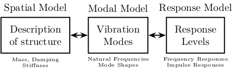
Figure 6: Vibration Analysis Procedure

The extraction of the Spatial Model (3rd step) was not performed as it requires a lot of time and was not judge necessary.

2.1 Setup

To measure the dynamics of such complicated system, it as been chosen to perform a modal analysis.

To limit the number of degrees of freedom to be measured, we suppose that in the frequency range of interest (DC-300Hz), each of the positioning stage is behaving as a solid body. Thus, to fully describe the dynamics of the station, we (only) need to measure 6 degrees of freedom on each of the positioning stage (that is 36 degrees of freedom for the 6 solid bodies).

In order to perform the Modal Analysis, the following devices were used:

An acquisition system (OROS) with 24bits ADCs
3 tri-axis Accelerometers
An Instrumented Hammer

The measurement thus consists of:

Exciting the structure at the same location with the Hammer (Figure 7)
Move the accelerometers to measure all the DOF of the structure. The position of the accelerometers are:
- 4 on the first granite
- 4 on the second granite
- 4 on top of the translation stage (figure 8)
- 4 on top of the tilt stage
- 3 on top of the spindle
- 4 on top of the hexapod

In total, 69 degrees of freedom are measured (23 tri axis accelerometers) which is more that what was required.

We chose to have some redundancy in the measurement to be able to verify that the solid-body assumption is correct for each of the stage.

Figure 7: Example of one hammer impact

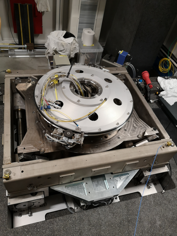
Figure 8: 3 tri axis accelerometers fixed to the translation stage

2.2 Results

From the measurements, we obtain all the transfer functions from forces applied at the location of the hammer impacts to the x-y-z acceleration of each solid body at the location of each accelerometer.

Modal shapes and natural frequencies are then computed. Example of mode shapes are shown in Figures 9 10.

Figure 9: First mode that shows a suspension mode, probably due to bad leveling of one Airloc

Figure 10: Sixth mode

We then reduce the number of degrees of freedom from 69 (23 accelerometers with each 3DOF) to 36 (6 solid bodies with 6 DOF).

From the reduced transfer function matrix, we can re-synthesize the response at the 69 measured degrees of freedom and we find that we have an exact match.

This confirms the fact that the stages are indeed behaving as a solid body in the frequency band of interest. This thus means that a multi-body model can be used to represent the dynamics of the micro-station.

Many Frequency Response Functions (FRF) are obtained from the measurements. Examples of FRF are shown in Figure 11. These FRF will be used to compare the dynamics of the multi-body model with the micro-station dynamics.

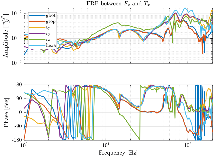
Figure 11: Frequency Response Function from forces applied by the Hammer in the X direction to the acceleration of each solid body in the X direction

2.3 Conclusion

The modal analysis of the micro-station confirmed the fact that a multi-body model should be able to correctly represents the micro-station dynamics. In Section 4, the obtained Frequency Response Functions will be used to compare the model dynamics with the micro-station dynamics.

3 Identification of the Disturbances

In this section, we wish to list and identify all the disturbances affecting the system.

Note that here we are not much interested by low frequency disturbances such as thermal effects and static guiding errors of each positioning stage. This is because the frequency content of these errors will be located in the controller bandwidth and thus will be easily compensated by the nano-hexapod.

The problem are on the high frequency disturbances. In the following sections, we consider:

the ground motion
vibrations of each stage, due either to their control systems or their motion

https://tdehaeze.github.io/meas-analysis/ Open Loop Noise budget: https://tdehaeze.github.io/nass-simscape/disturbances.html

3.1 Ground Motion

The ground motion can easily be estimated using an inertial sensor with sufficient sensitivity.

To verify that the inertial sensors are sensitive enough, a Huddle test has been performed (Figure 12).

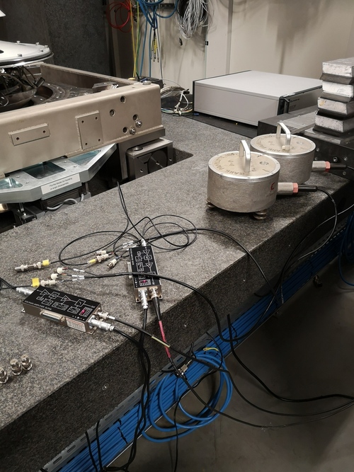
Figure 12: Huddle Test Setup

The measured Power Spectral Density of the ground motion at the ID31 floor is compared with other measurements performed at ID09 and at CERN. The low frequency differences between the ground motion at ID31 and ID09 is just due to the fact that for the later measurement, the low frequency sensitivity of the inertial sensor was not taken into account.

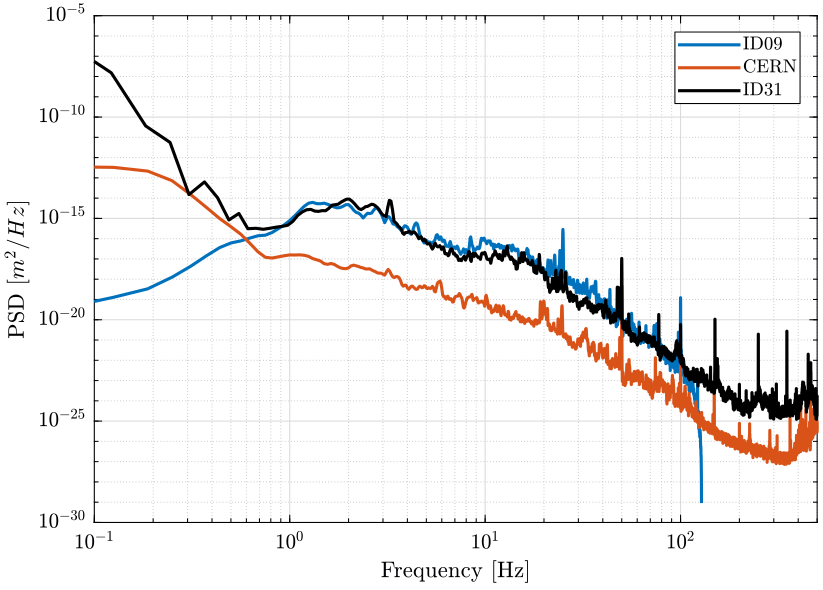
Figure 13: Comparison of the PSD of the ground motion measured at different location

3.2 Stage Vibration - Effect of Control systems

Control system of each stage has been tested

Each motor are turn off and then on. The goal is to see what noise is injected in the system due to the regulation loop of each stage.

Complete reports on these measurements are accessible here and here.

25Hz vertical motion when the Spindle is turned on (even when not rotating).

3.3 Stage Vibration - Effect of Motion

We consider here the vibrations induced by the scans of the translation stage and rotation of the spindle.

Details reports are accessible here for the translation stage and here for the spindle/slip-ring.

Spindle and Slip-Ring

The setup for the measurement of vibrations induced by rotation of the Spindle and Slip-ring is shown in Figure 14.

Figure 14: Measurement of the sample’s vertical motion when rotating at 6rpm

A geophone is fixed at the location of the sample and we measure the motion:

without rotation
when rotating at 6rpm using the slip-ring motor
when rotating at 6rpm using the spindle motor synchronized with the slip-ring motor

The obtained Power Spectral Density of the sample’s absolute velocity are shown in Figure 15.

We can see that when using the Slip-ring motor to rotate the sample, only a little increase of the motion is observed above 100Hz.

However, when rotating with the Spindle (normal functioning mode):

a very sharp peak at 23Hz is observed. Its cause has not been identified yet
a general large increase in motion above 30Hz

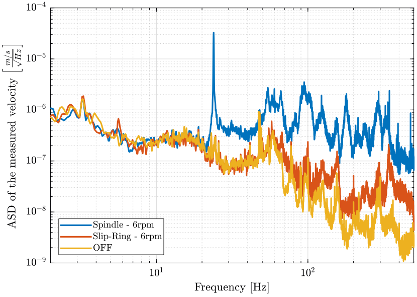
Figure 15: Comparison of the ASD of the measured voltage from the Geophone at the sample location

Some investigation should be performed on the Spindle to determine where does this 23Hz motion comes from.

Translation Stage

The same setup is used (a geophone is located at the sample’s location and another on the granite).

We impose a 1Hz triangle motion with an amplitude of \(\pm 2.5mm\) on the translation stage (Figure 16), and we measure the absolute velocity of both the sample and the granite.

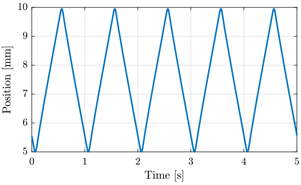
Figure 16: Y position of the translation stage measured by the encoders

The time domain absolute vertical velocity of the sample and granite are shown in Figure 17. It is shown that quite large motion of the granite is induced by the translation stage scans. This could be a problem if this is shown to excite the metrology frame of the nano-focusing lens position stage.

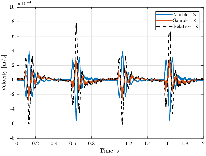
Figure 17: Vertical velocity of the sample and marble when scanning with the translation stage

The Amplitude Spectral Densities of the measured absolute velocities are shown in Figure 18. We can see many peaks starting from 1Hz showing the large spectral content probably due to the triangular reference of the translation stage.

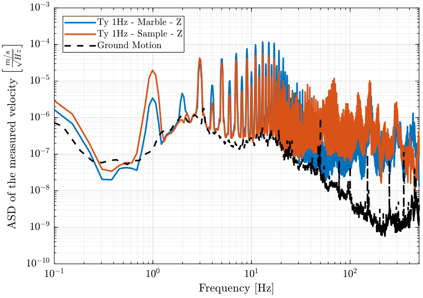
Figure 18: Amplitude spectral density of the measure velocity corresponding to the geophone in the vertical direction located on the granite and at the sample location when the translation stage is scanning at 1Hz

A smoother motion for the translation stage (such as a sinus motion) could probably help reducing much of the vibrations produced.

3.4 Sum of all disturbances

We can now compare the effect of all the disturbance sources on the position error (relative motion of the sample with respect to the granite).

The Power Spectral Density of the motion error due to the ground motion, translation stage scans and spindle rotation are shown in Figure 19.

We can see that the ground motion is quite small compare to the translation stage and spindle induced motions.

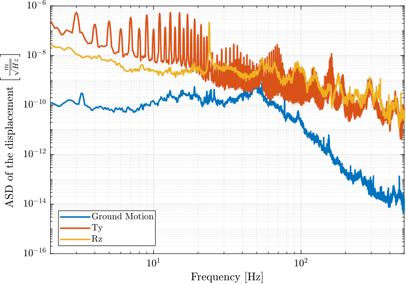
Figure 19: Amplitude Spectral Density fo the motion error due to disturbances

The Cumulative Amplitude Spectrum is shown in Figure 20. It is shown that the motion induced by translation stage scans and spindle rotation are in the micro-meter range.

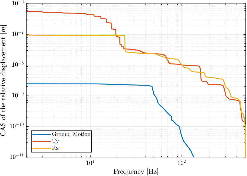
Figure 20: Cumulative Amplitude Spectrum of the motion error due to disturbances

We can also estimate the required bandwidth by seeing that \(10\ nm [rms]\) motion is induced by the perturbations above 100Hz.

This means that if the controller compensate all the motion errors below 100Hz (ideal case), 10nm [rms] of motion will still remain.

From that, we can conclude that we will probably need a control bandwidth to around 100Hz.

3.5 Better estimation of the disturbances

All the disturbance measurements were made with inertial sensors, and to obtain the relative motion sample/granite, two inertial sensors were used and the signals were subtracted.

This is not perfect as using only one geophone on the sample and one on the granite do not permit to separate the translations and the rotations.

An alternative could be to position a reference object at the sample location and to use the X-ray to measure its motion.

The detector requirement would be:

Sample frequency above \(400Hz\)
Resolution of \(\approx 100nm\) (to be discussed)

3.6 Conclusion

Main disturbance sources have been identified. These disturbances will then be included in the multi-body model.

Other disturbance sources were not estimated such as cable forces and acoustic disturbances. If heavy/stiff cables are to be fixed to the sample, this should be quantified and included in the model.

Having better estimation of the disturbances would allows to more precisely estimate the attainable performances. This should however not change the conclusion of this study nor significantly change the nano-hexapod design.

4 Multi Body Model

As was shown during the modal analysis (Section 2), the micro-station behaves as multiple rigid bodies (granite, translation stage, tilt stage, spindle, hexapod) with some discrete flexibility between those solid bodies.

Thus, a multi-body model is perfect to represent such dynamics.

To do so, we use the Matlab’s Simscape toolbox. A small summary of the multi-body Simscape is available here and each of the modeled stage is described here.

4.1 Multi-Body model

The mass/inertia of each stage is automatically computed from the imported geometry and the material’s density.

The (6dof) stiffness between two solid bodies is first guessed from either measurements of data-sheets. Then, the values of the stiffness and damping of each joint is manually tuned until the obtained dynamics is sufficiently close to the measured dynamics.

The 3D representation of the simscape model is shown in Figure 21.

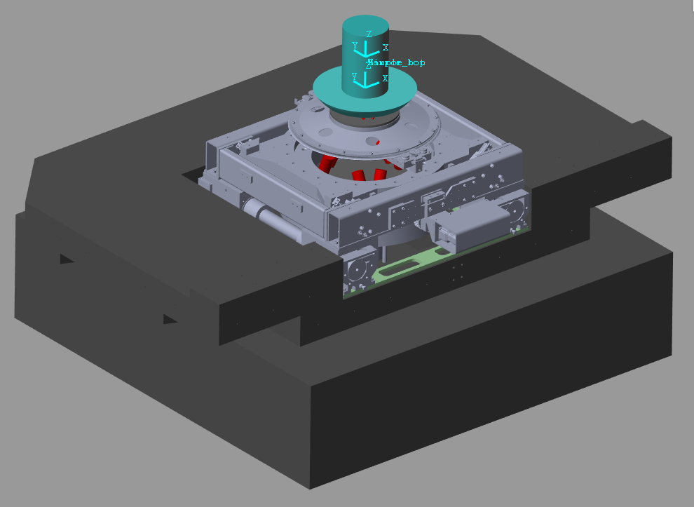
Figure 21: 3D representation of the simscape model

4.2 Validity of the model’s dynamics

It is very difficult the tune the dynamics of such model as there are more than 50 parameters and many curves to compare between the model and the measurements.

The comparison of three of the Frequency Response Functions are shown in Figure 22.

Most of the other measured FRFs and identified transfer functions from the multi-body model have the same level of matching.

We believe that the model is representing the micro-station dynamics with sufficient precision for the current analysis.

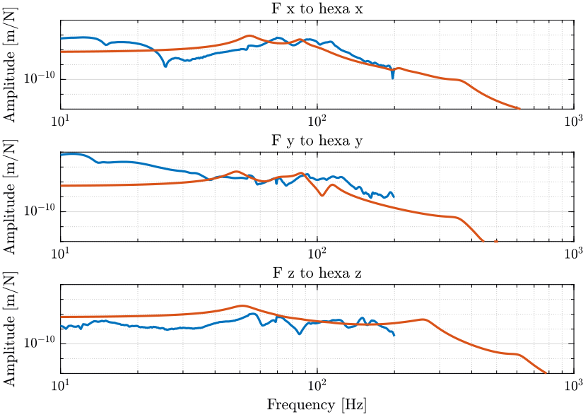
Figure 22: Frequency Response function from Hammer force in the X,Y and Z directions to the X,Y and Z displacements of the micro-hexapod’s top platform. The measurements are shown in blue and the Model in red.

More detailed comparison between the model and the measured dynamics is performed here.

Now that the multi-body model dynamics as been tuned, the following elements are included:

Actuators to perform the motion of each stage (translation, tilt, spindle, hexapod)
Sensors to measure the motion of each stage and the relative motion of the sample with respect to the granite (metrology system)
Disturbances such as ground motion and stage’s vibrations

Then, using the model, we can

perform simulation of experiments in presence of disturbances
measure the motion of the solid-bodies
identify the dynamics from inputs (forces, imposed displacement) to outputs (measured motion, force sensor, etc.) which will be useful for the nano-hexapod and control design
include a multi-body model of the nano-hexapod and closed-loop simulations

4.3 Wanted position of the sample and position error

For the control of the nano-hexapod, we need to now the sample position error (the motion to be compensated) in the frame of the nano-hexapod.

To do so, we need to perform several computations (summarized in Figure 23):

First, we need to determine the actual wanted pose (3 translations and 3 rotations) of the sample with respect to the granite. This is determined from the wanted motion of each micro-station stage. Each wanted stage motion is represented by an homogeneous transformation matrix (explain here), then these matrices are combined to give to total wanted motion of the sample with respect to the granite.
Then, we need to determine the actual pose of the sample with respect to the granite. This will be performed by several interferometers and several computation will be required to compute the pose of the sample from the interferometers measurements. However we here directly measure the 3 translations and 3 rotations of the sample using a special simscape block.
Finally, we need to compare the wanted pose with the measured pose to compute the position error of the sample. This position error can be expressed in the frame of the granite, or in the frame of the (rotating) nano-hexapod. Both computation are performed.

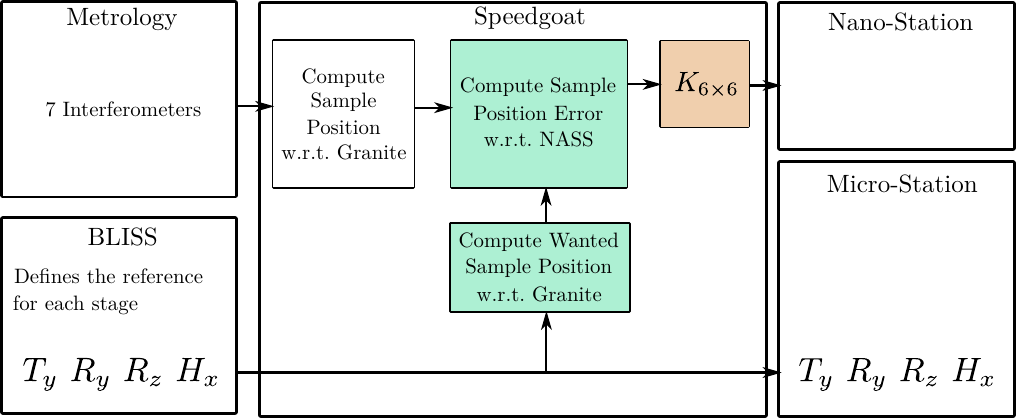
Figure 23: Figure caption

More details about these computations are accessible here.

4.4 Simulation of Experiments

Now that the dynamics of the model is tuned and the disturbances included in the model, we can perform simulation of experiments.

We first do a simulation where the nano-hexapod is considered to be a solid-body to estimate the sample’s motion that we have without an control.

An animation of the obtained motion is shown in Figure 24. A zoom in the micro-meter ranger on the sample’s location is shown in Figure 25.

Two frames are displayed:

a non-rotating frame that corresponds to the wanted position of the sample. Note that here this frame is moving with the granite.
a rotating frame that corresponds to the actual pose of the sample

Figure 24: Tomography Experiment using the Simscape Model

Figure 25: Tomography Experiment using the Simscape Model - Zoom on the sample’s position (the full vertical scale is \(\approx 10 \mu m\))

The position error of the sample with respect to the granite are shown in Figure 26. It is shown that the X-Y-Z position errors are in the micro-meter range.

For the rotation around X and Y, the errors are quite small. This is explained by the fact that no torque disturbances is considered in the model.

For the vertical rotation, this is due to the fact that we suppose perfect rotation of the Spindle, and anyway, no measurement of the sample with respect to the granite is made by the interferometers.

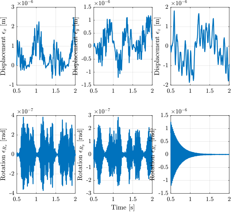
Figure 26: Position error of the Sample with respect to the granite during a Tomography Experiment with included disturbances

4.5 Conclusion

The multi-body model developed using Simscape is shown to be sufficiently close to the micro-station dynamics.

It makes possible to:

study many effects such as the change of dynamics due to the rotation, the sample mass, etc.
extract transfer function like \(G\) and \(G_d\)
simulate experiments to validate performance

This model will be used in the next sections to help the design of the nano-hexapod, to develop the robust control architecture and to perform simulation in order to validate.

5 Optimal Nano-Hexapod Design

As explain before, the nano-hexapod properties (mass, stiffness, architecture, …) will influence:

the effect of disturbances \(G_d\) (important for the rejection of disturbances)
the plant dynamics \(G\) (important for the control robustness properties)

Thus, we here wish to find the optimal nano-hexapod properties such that:

the effect of disturbances is minimized (Section 5.1)
the plant uncertainty due to a change of payload mass and experimental conditions is minimized (Section 5.2)

The study presented here only consider changes in the nano-hexapod stiffness for two reasons:

the nano-hexapod mass cannot be change too much, and will anyway be negligible compare to the metrology reflector and the payload masses
the choice of the nano-hexapod architecture (e.g. orientations of the actuators and implementation of sensors) will be further studied in accord with the control architecture

5.1 Optimal Stiffness to reduce the effect of disturbances

As will be seen, the nano-hexapod stiffness have a large influence on the sensibility to disturbance (the norm of \(G_d\)). For instance, it is quite obvious that a stiff nano-hexapod is better than a soft one when it comes to direct forces applied to the sample such as cable forces.

A complete study of the optimal nano-hexapod stiffness for the minimization of disturbance sensibility here and summarized below.

The sensibility to the spindle’s vibration for all the considered nano-hexapod stiffnesses (from \(10^3\,[N/m]\) to \(10^9\,[N/m]\)) is shown in Figure 27. It is shown that a softer nano-hexapod it better to filter out vertical vibrations of the spindle. More precisely, is start to filters the vibration at the first suspension mode of the payload on top of the nano-hexapod.

The same conclusion is made for vibrations of the translation stage.

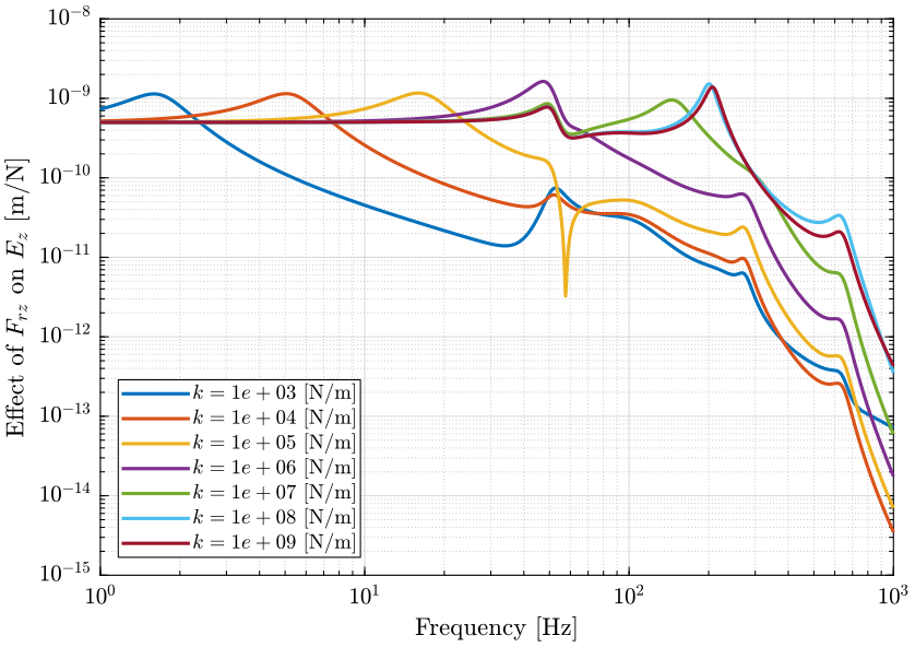
Figure 27: Sensitivity to Spindle vertical motion error to the vertical error position of the sample

The sensibilities to ground motion in the Y and Z directions are shown in Figure 28. We can see that above the suspension mode of the nano-hexapod, the norm of the transmissibility is close to one until the suspension mode of the granite. Thus, a stiff nano-hexapod is better for reducing the effect of ground motion at low frequency.

It will be further suggested that using soft mounts for the granite can greatly lower the sensibility to ground motion.

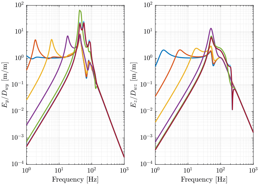
Figure 28: Sensitivity to Ground motion to the position error of the sample

However, lowering the sensibility to some disturbance at a frequency where its effect is already small compare to the other disturbances sources is not really interesting. What is more important than comparing the sensitivity to disturbances, is thus to compare the obtain power spectral density of the sample’s position error. From the Power Spectral Density of all the sources of disturbances identified in Section 3, we compute what would be the Power Spectral Density of the vertical motion error for all the considered nano-hexapod stiffnesses (Figure 29).

We can see that the most important change is in the frequency range 30Hz to 300Hz where a stiffness smaller than \(10^5\,[N/m]\) greatly reduces the sample’s vibrations.

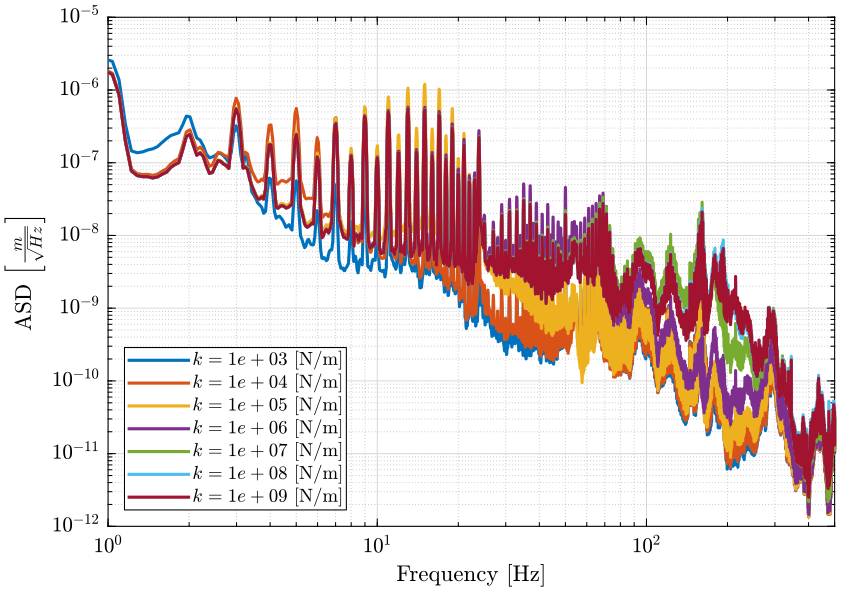
Figure 29: Amplitude Spectral Density of the Sample vertical position error due to Vertical vibration of the Spindle for multiple nano-hexapod stiffnesses

If we look at the Cumulative amplitude spectrum of the vertical error motion in Figure 30, we can observe that a soft hexapod (\(k < 10^5 - 10^6\,[N/m]\)) helps reducing the high frequency disturbances, and thus a smaller control bandwidth will suffice to obtain the wanted performance.

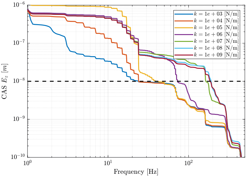
Figure 30: Cumulative Amplitude Spectrum of the Sample vertical position error due to all considered perturbations for multiple nano-hexapod stiffnesses

5.2 Optimal Stiffness to reduce the plant uncertainty

One of the most important design goal is to obtain a system that is robust to all changes in the system. Therefore, we have to identify all changes that might occurs in the system and choose the nano-hexapod stiffness such that the uncertainty to these changes is minimized.

The uncertainty in the system can be caused by:

A change in the Support’s compliance (complete analysis here): if the micro-station dynamics is changing due to the change of parts or just because of aging effects, the feedback system should remains stable and the obtained performance should not change
A change in the Payload mass/dynamics (complete analysis here): the sample’s mass is ranging from \(1\,kg\) to \(50\,kg\)
A change of experimental condition such as the micro-station’s pose or the spindle rotation (complete analysis here)

All these uncertainties will limit the attainable bandwidth and hence the obtained performance.

In the next sections, the effect of each change on the obtained uncertainty is quantified and conclusions are made on the optimal stiffness for robustness properties.

Note that only the dynamics from forces applied by the nano-hexapod to the measured sample’s position by the metrology are compared. This is because it is the most important dynamics for robustness and performance properties. However, the dynamics from forces to sensors located in the nano-hexapod legs, such as force and relative motion sensors, have also been considered.

Effect of Payload

The most obvious change in the system is the change of payload.

In Figure

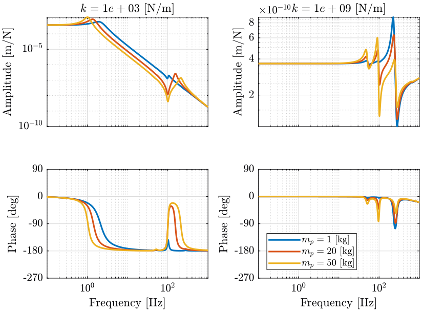
Figure 31: Dynamics from \(\mathcal{F}_z\) to \(\mathcal{X}_z\) for varying payload mass, both for a soft nano-hexapod and a stiff nano-hexapod

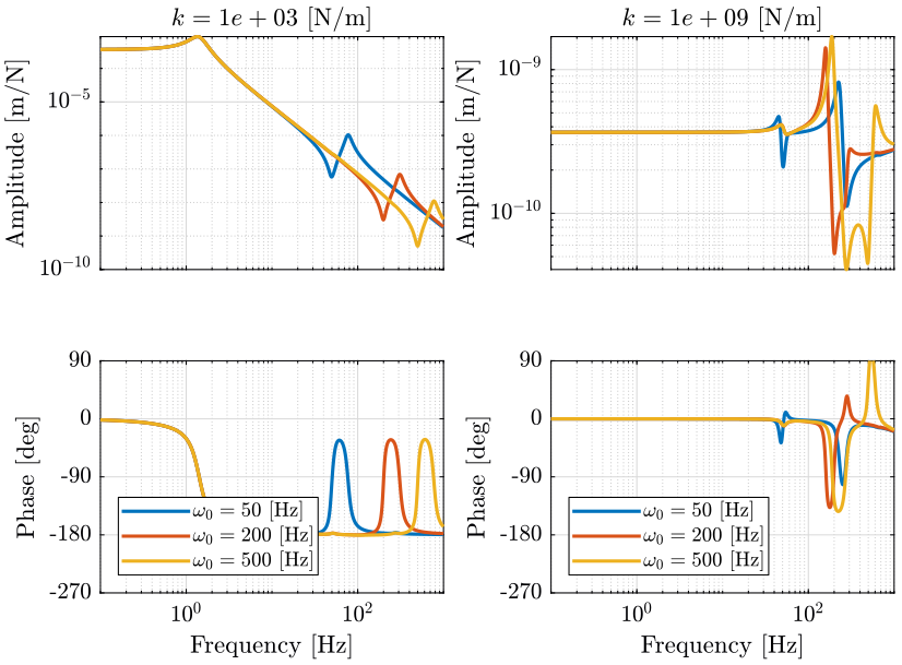
Figure 32: Dynamics from \(\mathcal{F}_z\) to \(\mathcal{X}_z\) for varying payload resonance frequency, both for a soft nano-hexapod and a stiff nano-hexapod

Effect of Micro-Station Compliance

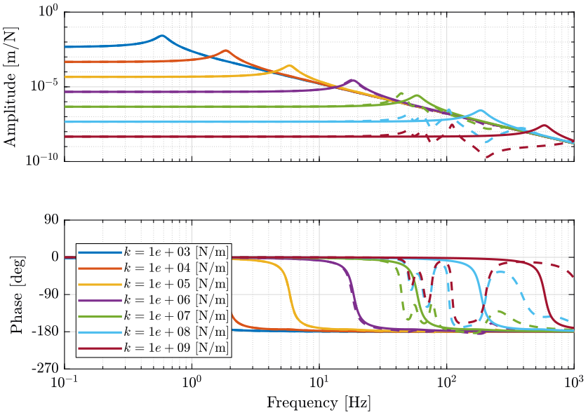
Figure 33: Change of dynamics from force \(\mathcal{F}_x\) to displacement \(\mathcal{X}_x\) due to the micro-station compliance

Effect of Spindle Rotating Speed

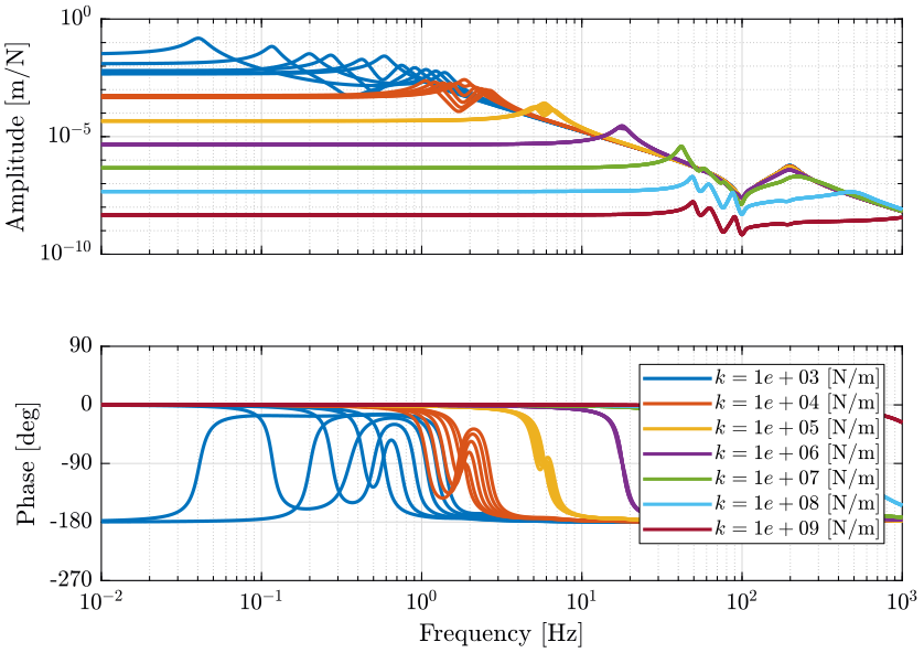
Figure 34: Change of dynamics from force \(\mathcal{F}_x\) to displacement \(\mathcal{X}_x\) for a spindle rotation speed from 0rpm to 60rpm

Total Uncertainty

Figure 35: Variability of the dynamics from \(\bm{\mathcal{F}}_x\) to \(\bm{\mathcal{X}}_x\) with varying nano-hexapod stiffness

The leg stiffness should be at higher than \(k = 10^4\,[N/m]\) such that the main resonance frequency does not shift too much when rotating.

It is usually a good idea to maximize the mass, damping and stiffness of the isolation platform in order to be less sensible to the payload dynamics. The best thing to do is to have a stiff isolation platform.

The dynamics of the nano-hexapod is not affected by the micro-station dynamics (compliance) when the stiffness of the legs is less than \(10^6\,[N/m]\). When the nano-hexapod is stiff (\(k > 10^7\,[N/m]\)), the compliance of the micro-station appears in the primary plant.

Determination of the optimal stiffness based on all the effects:

https://tdehaeze.github.io/nass-simscape/uncertainty_optimal_stiffness.html

The main performance limitation are payload variability

Main problem: heavy samples with small stiffness. The first resonance frequency of the sample will limit the performance.

It is preferred that one controller is working for all the payloads. If not possible, the alternative would be to develop an adaptive controller that depends on the payload mass/inertia.

5.3 Conclusion

6 Robust Control Architecture

https://tdehaeze.github.io/nass-simscape/optimal_stiffness_control.html

6.1 Active Damping and Sensors to be included

Ways to damp:

Force Sensor
Relative Velocity Sensors
Inertial Sensor

https://tdehaeze.github.io/rotating-frame/index.html

Sensors to be included:

6.2 Motion Control

6.3 Simulation of Tomography Experiments

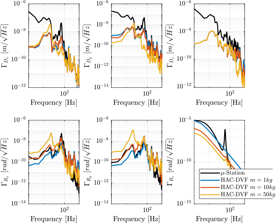
Figure 36: Amplitude Spectral Density of the position error in Open Loop and with the HAC-LAC controller

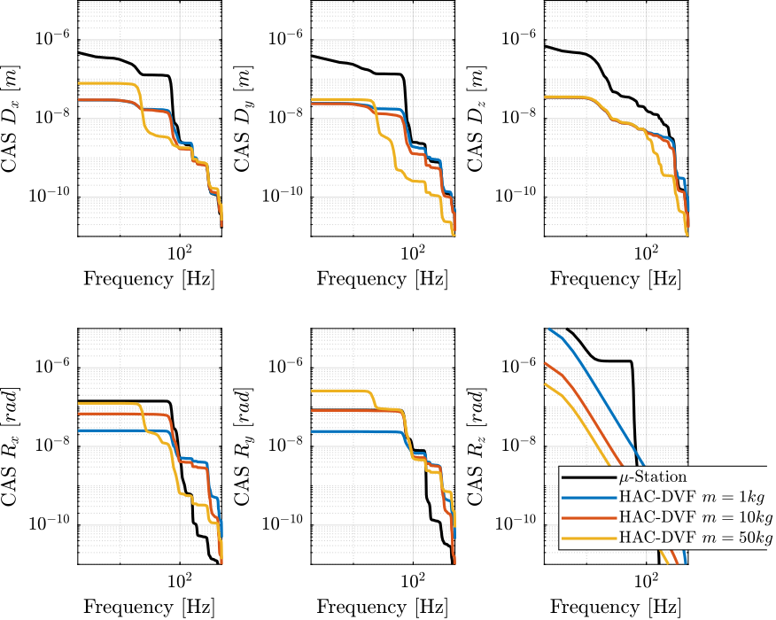
Figure 37: Cumulative Amplitude Spectrum of the position error in Open Loop and with the HAC-LAC controller

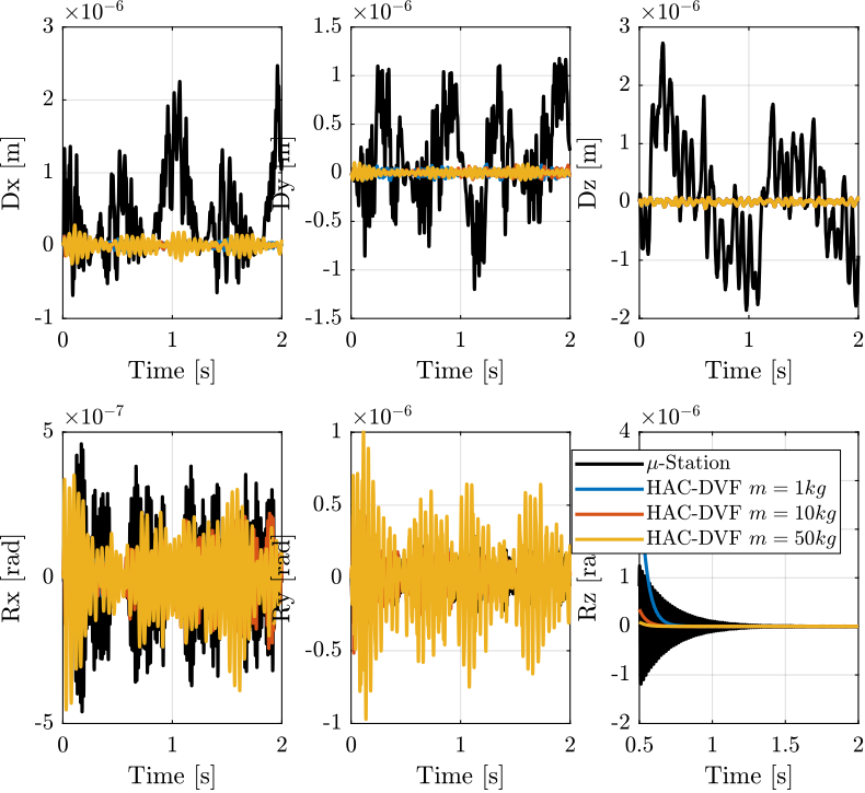
Figure 38: Position Error of the sample during a tomography experiment when no control is applied and with the HAC-DVF control architecture

Figure 39: Tomography Experiment using the Simscape Model in Closed Loop with the HAC-LAC Control - Zoom on the sample’s position (the full vertical scale is \(\approx 10 \mu m\))

6.4 Conclusion

7 Further notes

Soft granite

Sensible to detector motion?

Common metrology frame for the nano-focusing optics and the measurement of the sample position?

Cable forces?

Slip-Ring noise?

Bibliography

[schmidt14_desig_high_perfor_mechat_revis_edition] Schmidt, Schitter & Rankers, The Design of High Performance Mechatronics - 2nd Revised Edition, Ios Press (2014).
[oomen18_advan_motion_contr_precis_mechat] Tom Oomen, Advanced Motion Control for Precision Mechatronics: Control, Identification, and Learning of Complex Systems, IEEJ Journal of Industry Applications, 7(2), 127-140 (2018). link. doi.