Modal Analysis - Modal Parameter Extraction
Table of Contents
- 1. Load Data
- 2. Determine the number of modes
- 3. Modal parameter extraction
- 4. Obtained Mode Shapes animations
- 5. Verify the validity of the Modal Model
- 6. Modal Complexity
- 7. Modal Assurance Criterion (MAC)
- 8. From accelerometer coordinates to global coordinates for the mode shapes
- 9. Some notes about constraining the number of degrees of freedom
- 10. Compare Mode Shapes
- 11. TODO Mode shapes expressed in a frame at the CoM of the solid bodies
- 12. TODO Residues
The goal here is to extract the modal parameters describing the modes of station being studied, namely:
- the eigen frequencies and the modal damping (eigen values)
- the mode shapes (eigen vectors)
This is done from the FRF matrix previously extracted from the measurements.
In order to do the modal parameter extraction, we first have to estimate the order of the modal model we want to obtain. This corresponds to how many modes are present in the frequency band of interest. In section 2, we will use the Singular Value Decomposition and the Modal Indication Function to estimate the number of modes.
The modal parameter extraction methods generally consists of curve-fitting a theoretical expression for an individual FRF to the actual measured data. However, there are multiple level of complexity:
- works on a part of a single FRF curve
- works on a complete curve encompassing several resonances
- works on a set of many FRF plots all obtained from the same structure
The third method is the most complex but gives better results. This is the one we will use in section 3.
From the modal model, it is possible to obtain a graphic display of the mode shapes (section 4).
In order to validate the quality of the modal model, we will synthesize the FRF matrix from the modal model and compare it with the FRF measured (section 5).
The modes of the structure are expected to be complex, however real modes are easier to work with when it comes to obtain a spatial model from the modal parameters. We will thus study the complexity of those modes, in section 6, and see if we can estimate real modes from the complex modes.
The mode obtained from the modal software describe the motion of the structure at the position of each accelerometer for all the modes. However, we would like to describe the motion of each stage (solid body) of the structure in its 6 DOFs. This in done in section 8.
Residues will have to be included.
All the files (data and Matlab scripts) are accessible here.
1 Load Data
load('mat/frf_coh_matrices.mat', 'FRFs', 'COHs', 'freqs');
load('mat/geometry.mat', 'solids', 'solid_names', 'acc_pos');
load('mat/frf_o.mat', 'FRFs_O');
2 Determine the number of modes
2.1 Singular Value Decomposition - Modal Indication Function
The Mode Indicator Functions are usually used on \(n\times p\) FRF matrix where \(n\) is a relatively large number of measurement DOFs and \(p\) is the number of excitation DOFs, typically 3 or 4.
In these methods, the frequency dependent FRF matrix is subjected to a singular value decomposition analysis which thus yields a small number (3 or 4) of singular values, these also being frequency dependent.
These methods are used to determine the number of modes present in a given frequency range, to identify repeated natural frequencies and to pre process the FRF data prior to modal analysis.
From the documentation of the modal software:
The MIF consist of the singular values of the Frequency response function matrix. The number of MIFs equals the number of excitations. By the powerful singular value decomposition, the real signal space is separated from the noise space. Therefore, the MIFs exhibit the modes effectively. A peak in the MIFs plot usually indicate the existence of a structural mode, and two peaks at the same frequency point means the existence of two repeated modes. Moreover, the magnitude of the MIFs implies the strength of the a mode.
The Complex Mode Indicator Function is defined simply by the SVD of the FRF (sub) matrix:
\begin{align*} [H(\omega)]_{n\times p} &= [U(\omega)]_{n\times n} [\Sigma(\omega)]_{n\times p} [V(\omega)]_{p\times p}^H\\ [CMIF(\omega)]_{p\times p} &= [\Sigma(\omega)]_{p\times n}^T [\Sigma(\omega)]_{n\times p} \end{align*}We compute the Complex Mode Indicator Function. The result is shown on figure 1. The exact same curve is obtained when computed using the OROS software.
MIF = zeros(size(FRFs, 2), size(FRFs, 2), size(FRFs, 3));

for i = 1:length(freqs)
  [~,S,~] = svd(FRFs(:, :, i));
  MIF(:, :, i) = S'*S;
end
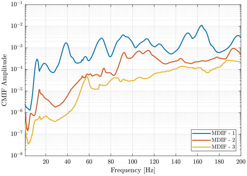
Figure 1: Complex Mode Indicator Function
We can also compute the CMIF using the FRF matrix expressed in the same global frame. We compare the two CMIF on figure 2.
They do not indicate the same resonance frequencies, especially around 110Hz.
MIF_O = zeros(size(FRFs_O, 2), size(FRFs_O, 2), size(FRFs_O, 3));
for i = 1:length(freqs)
  [~,S,~] = svd(FRFs_O(:, :, i));
  MIF_O(:, :, i) = S'*S;
end
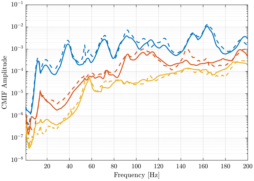
Figure 2: Complex Mode Indicator Function - Original FRF: solid curves - Processed FRF: dashed curve
2.2 Composite Response Function
An alternative is the Composite Response Function \(HH(\omega)\) defined as the sum of all the measured FRF:
\begin{equation} HH(\omega) = \sum_j\sum_kH_{jk}(\omega) \end{equation}Instead, we choose here to use the sum of the norms of the measured FRFs:
\begin{equation} HH(\omega) = \sum_j\sum_k \left|H_{jk}(\omega) \right| \end{equation}The result is shown on figure 3.
figure;
hold on;
plot(freqs, squeeze(sum(sum(abs(FRFs)))), '-k');
plot(freqs, squeeze(sum(sum(abs(FRFs_O)))), '--k');
hold off;
xlabel('Frequency [Hz]'); ylabel('Amplitude');
xlim([1, 200]);
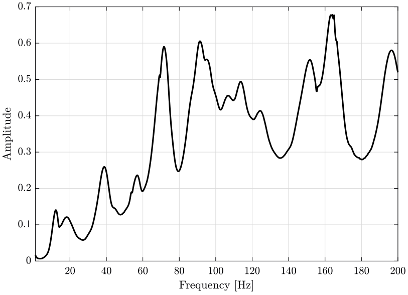
Figure 3: Composite Response Function. Solid curve: computed from the original FRFs. Dashed curve: computed from the FRFs expressed in the global frame.
3 Modal parameter extraction
3.1 OROS - Modal software
Modal identification are done within the Modal software of OROS. The manual for the software is available here.
Several modal parameter extraction methods are available. We choose to use the "broad band" method as it permits to identify the modal parameters using all the FRF curves at the same time. It takes into account the fact the the properties of all the individual curves are related by being from the same structure: all FRF plots on a given structure should indicate the same values for the natural frequencies and damping factor of each mode.
Such method also have the advantage of producing a unique and consistent model as direct output.
In order to apply this method, we select the frequency range of interest and we give an estimate of how many modes are present.
Then, it shows a stabilization charts, such as the one shown on figure 4, where we have to manually select which modes to take into account in the modal model.
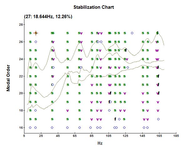
Figure 4: Stabilization Chart
We can then run the modal analysis, and the software will identify the modal damping and mode shapes at the selected frequency modes.
3.2 Exported modal parameters
The obtained modal parameters are:
- resonance frequencies in Hertz
- modal damping ratio in percentage
- (complex) modes shapes for each measured DoF
- modal A and modal B which are parameters important for further normalization
They are all exported in a text file named modes.asc.
Its first 20 lines as shown below.
Created by N-Modal
Estimator: bbfd
01-Jul-19 16:44:11


Mode 1
freq    = 11.41275Hz
damp    = 8.72664%
modal A =  -4.50556e+003-9.41744e+003i
modal B =  -7.00928e+005+2.62922e+005i
Mode matrix of local coordinate [DOF: Re IM]
     1X-:  -1.04114e-001   3.50664e-002
     1Y-:   2.34008e-001   5.04273e-004
     1Z+:  -1.93303e-002   5.08614e-003
     2X-:  -8.38439e-002   3.45978e-002
     2Y-:   2.42440e-001   0.00000e+000
     2Z+:  -7.40734e-003   5.17734e-003
     3Y-:   2.17655e-001   6.10802e-003
     3X+:   1.18685e-001  -3.54602e-002
     3Z+:  -2.37725e-002  -1.61649e-003
We split this big modes.asc file into sub text files using bash. The obtained files are described one table 1.
sed '/^\s*[0-9]*[XYZ][+-]:/!d' mat/modes.asc > mat/mode_shapes.txt
sed '/freq/!d'                 mat/modes.asc | sed 's/.* = \(.*\)Hz/\1/' > mat/mode_freqs.txt
sed '/damp/!d'                 mat/modes.asc | sed 's/.* = \(.*\)\%/\1/' > mat/mode_damps.txt
sed '/modal A/!d'              mat/modes.asc | sed 's/.* =\s\+\([-0-9.e]\++[0-9]\+\)\([-+0-9.e]\+\)i/\1 \2/' > mat/mode_modal_a.txt
sed '/modal B/!d'              mat/modes.asc | sed 's/.* =\s\+\([-0-9.e]\++[0-9]\+\)\([-+0-9.e]\+\)i/\1 \2/' > mat/mode_modal_b.txt
| Filename | Content |
|---|---|
mat/mode_shapes.txt |
mode shapes |
mat/mode_freqs.txt |
resonance frequencies [Hz] |
mat/mode_damps.txt |
modal damping [per] |
mat/mode_modal_a.txt |
Modal A |
mat/mode_modal_b.txt |
Modal B |
3.3 Importation of the modal parameters on Matlab
Then we import the obtained .txt files on Matlab using readtable function.
shapes_m = readtable('mat/mode_shapes.txt',              'ReadVariableNames', false);  % [Sign / Real / Imag]
freqs_m  = table2array(readtable('mat/mode_freqs.txt',   'ReadVariableNames', false)); % in [Hz]
damps_m  = table2array(readtable('mat/mode_damps.txt',   'ReadVariableNames', false)); % in [%]
modal_a  = table2array(readtable('mat/mode_modal_a.txt', 'ReadVariableNames', false)); % [Real / Imag]
modal_b  = table2array(readtable('mat/mode_modal_b.txt', 'ReadVariableNames', false)); % [Real / Imag]
We guess the number of modes identified from the length of the imported data.
acc_n = 23; % Number of accelerometers
dir_n = 3; % Number of directions
dirs = 'XYZ';

mod_n = size(shapes_m,1)/acc_n/dir_n; % Number of modes
As the mode shapes are split into 3 parts (direction plus sign, real part and imaginary part), we aggregate them into one array of complex numbers.
T_sign = table2array(shapes_m(:, 1));
T_real = table2array(shapes_m(:, 2));
T_imag = table2array(shapes_m(:, 3));

mode_shapes = zeros(mod_n, dir_n, acc_n);

for mod_i = 1:mod_n
  for acc_i = 1:acc_n
    % Get the correct section of the signs
    T = T_sign(acc_n*dir_n*(mod_i-1)+1:acc_n*dir_n*mod_i);
    for dir_i = 1:dir_n
      % Get the line corresponding to the sensor
      i = find(contains(T, sprintf('%i%s',acc_i, dirs(dir_i))), 1, 'first')+acc_n*dir_n*(mod_i-1);
      mode_shapes(mod_i, dir_i, acc_i) = str2num([T_sign{i}(end-1), '1'])*complex(T_real(i),T_imag(i));
    end
  end
end
The obtained mode frequencies and damping are shown below.
| Mode number | Frequency [Hz] | Damping [%] |
|---|---|---|
| 1.0 | 11.4 | 8.7 |
| 2.0 | 18.5 | 11.8 |
| 3.0 | 37.6 | 6.4 |
| 4.0 | 39.4 | 3.6 |
| 5.0 | 54.0 | 0.2 |
| 6.0 | 56.1 | 2.8 |
| 7.0 | 69.7 | 4.6 |
| 8.0 | 71.6 | 0.6 |
| 9.0 | 72.4 | 1.6 |
| 10.0 | 84.9 | 3.6 |
| 11.0 | 90.6 | 0.3 |
| 12.0 | 91.0 | 2.9 |
| 13.0 | 95.8 | 3.3 |
| 14.0 | 105.4 | 3.3 |
| 15.0 | 106.8 | 1.9 |
| 16.0 | 112.6 | 3.0 |
| 17.0 | 116.8 | 2.7 |
| 18.0 | 124.1 | 0.6 |
| 19.0 | 145.4 | 1.6 |
| 20.0 | 150.1 | 2.2 |
| 21.0 | 164.7 | 1.4 |
3.4 Theory
It seems that the modal analysis software makes the assumption of viscous damping for the model with which it tries to fit the FRF measurements.
If we note \(N\) the number of modes identified, then there are \(2N\) eigenvalues and eigenvectors given by the software:
\begin{align} s_r &= \omega_r (-\xi_r + i \sqrt{1 - \xi_r^2}),\quad s_r^* \\ \{\psi_r\} &= \begin{Bmatrix} \psi_{1_x} & \psi_{2_x} & \dots & \psi_{23_x} & \psi_{1_y} & \dots & \psi_{1_z} & \dots & \psi_{23_z} \end{Bmatrix}^T, \quad \{\psi_r\}^* \end{align}for \(r = 1, \dots, N\) where \(\omega_r\) is the natural frequency and \(\xi_r\) is the critical damping ratio for that mode.
3.5 Modal Matrices
We would like to arrange the obtained modal parameters into two modal matrices: \[ \Lambda = \begin{bmatrix} s_1 & & 0 \\ & \ddots & \\ 0 & & s_N \end{bmatrix}_{N \times N}; \quad \Psi = \begin{bmatrix} & & \\ \{\psi_1\} & \dots & \{\psi_N\} \\ & & \end{bmatrix}_{M \times N} \] \[ \{\psi_i\} = \begin{Bmatrix} \psi_{i, 1_x} & \psi_{i, 1_y} & \psi_{i, 1_z} & \psi_{i, 2_x} & \dots & \psi_{i, 23_z} \end{Bmatrix}^T \]
\(M\) is the number of DoF: here it is \(23 \times 3 = 69\). \(N\) is the number of mode
eigen_val_M = diag(2*pi*freqs_m.*(-damps_m/100 + j*sqrt(1 - (damps_m/100).^2)));
eigen_vec_M = reshape(mode_shapes, [mod_n, acc_n*dir_n]).';
Each eigen vector is normalized: \(\| \{\psi_i\} \|_2 = 1\)
However, the eigen values and eigen vectors appears as complex conjugates: \[ s_r, s_r^*, \{\psi\}_r, \{\psi\}_r^*, \quad r = 1, N \]
In the end, they are \(2N\) eigen values. We then build two extended eigen matrices as follow: \[ \mathcal{S} = \begin{bmatrix} s_1 & & & & & \\ & \ddots & & & 0 & \\ & & s_N & & & \\ & & & s_1^* & & \\ & 0 & & & \ddots & \\ & & & & & s_N^* \end{bmatrix}_{2N \times 2N}; \quad \Phi = \begin{bmatrix} & & & & &\\ \{\psi_1\} & \dots & \{\psi_N\} & \{\psi_1^*\} & \dots & \{\psi_N^*\} \\ & & & & & \end{bmatrix}_{M \times 2N} \]
eigen_val_ext_M = blkdiag(eigen_val_M, conj(eigen_val_M));
eigen_vec_ext_M = [eigen_vec_M, conj(eigen_vec_M)];
We also build the Modal A and Modal B matrices:
\begin{equation} A = \begin{bmatrix} a_1 & & 0 \\ & \ddots & \\ 0 & & a_N \end{bmatrix}_{N \times N}; \quad B = \begin{bmatrix} b_1 & & 0 \\ & \ddots & \\ 0 & & b_N \end{bmatrix}_{N \times N} \end{equation}With \(a_i\) is the "Modal A" parameter linked to mode i.
modal_a_M = diag(complex(modal_a(:, 1), modal_a(:, 2)));
modal_b_M = diag(complex(modal_b(:, 1), modal_b(:, 2)));

modal_a_ext_M = blkdiag(modal_a_M, conj(modal_a_M));
modal_b_ext_M = blkdiag(modal_b_M, conj(modal_b_M));
4 Obtained Mode Shapes animations
From the modal parameters, it is possible to show the modal shapes with an animation.
Examples are shown on figures 5 and 6.
Animations of all the other modes are accessible using the following links: mode 1, mode 2, mode 3, mode 4, mode 5, mode 6, mode 7, mode 8, mode 9, mode 10, mode 11, mode 12, mode 13, mode 14, mode 15, mode 16, mode 17, mode 18, mode 19, mode 20, mode 21.
Figure 5: Mode 1
Figure 6: Mode 6
We can learn quite a lot from these mode shape animations.
For instance, the mode shape of the first mode at 11Hz (figure 5) seems to indicate that this corresponds to a suspension mode.
This could be due to the 4 Airloc Levelers that are used for the granite (figure 7).
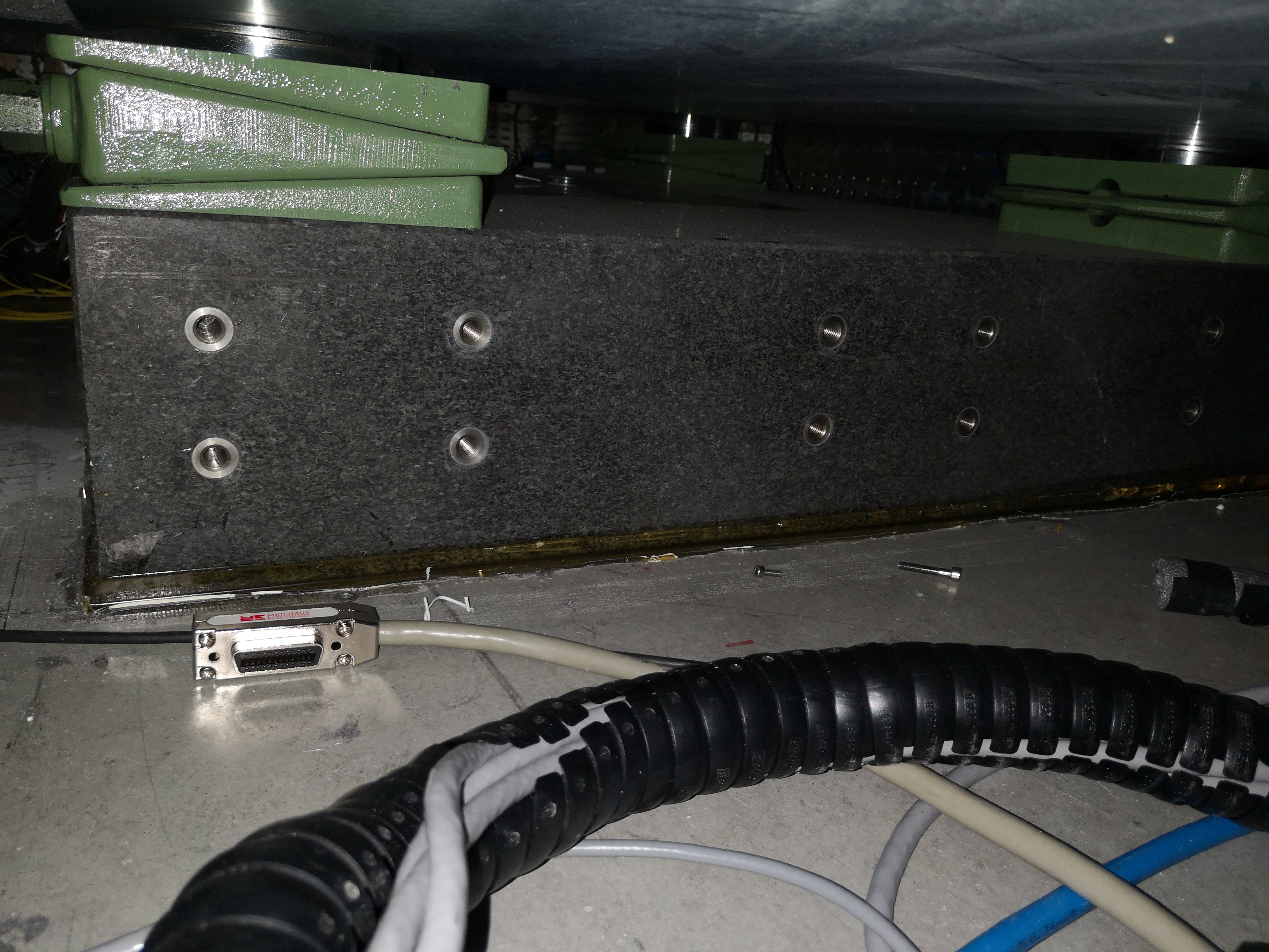
Figure 7: AirLoc used for the granite (2120-KSKC)
They are probably not well leveled, so the granite is supported only by two Airloc.
5 Verify the validity of the Modal Model
There are two main ways to verify the validity of the modal model
- Synthesize FRF measurements that has been used to generate the modal model and compare
- Synthesize FRF that has not yet been measured. Then measure that FRF and compare
5.1 Theory
From the modal model, we want to synthesize the Frequency Response Functions that has been used to build the modal model.
Let's recall that:
- \(M\) is the number of measured DOFs (\(23 \times 3 = 69\))
- \(N\) is the number of modes identified (\(21\))
We then have that the FRF matrix \([H_{\text{syn}}]\) can be synthesize using the following formula:
with \(Q_r = 1/M_{A_r}\)
An alternative formulation is: \[ H_{pq}(s_i) = \sum_{r=1}^N \frac{A_{pqr}}{s_i - \lambda_r} + \frac{A_{pqr}^*}{s_i - \lambda_r^*} \] with:
- \(A_{pqr} = \frac{\psi_{pr}\psi_{qr}}{M_{A_r}}\), \(M_{A_r}\) is called "Modal A"
- \(\psi_{pr}\): scaled modal coefficient for output DOF \(p\), mode \(r\)
- \(\lambda_r\): complex modal frequency
5.2 Matlab Implementation
Hsyn = zeros(69, 69, 801);

for i = 1:length(freqs)
  Hsyn(:, :, i) = eigen_vec_ext_M*(inv(modal_a_ext_M)/(diag(j*2*pi*freqs(i) - diag(eigen_val_ext_M))))*eigen_vec_ext_M.';
end
Because the synthesize frequency response functions are representing the displacement response in \([m/N]\), we multiply each element of the FRF matrix by \((j \omega)^2\) in order to obtain the acceleration response in \([m/s^2/N]\).
for i = 1:size(Hsyn, 1)
  Hsyn(i, :, :) = squeeze(-Hsyn(i, :, :)).*(j*2*pi*freqs).^2;
end
5.3 Original and Synthesize FRF matrix comparison
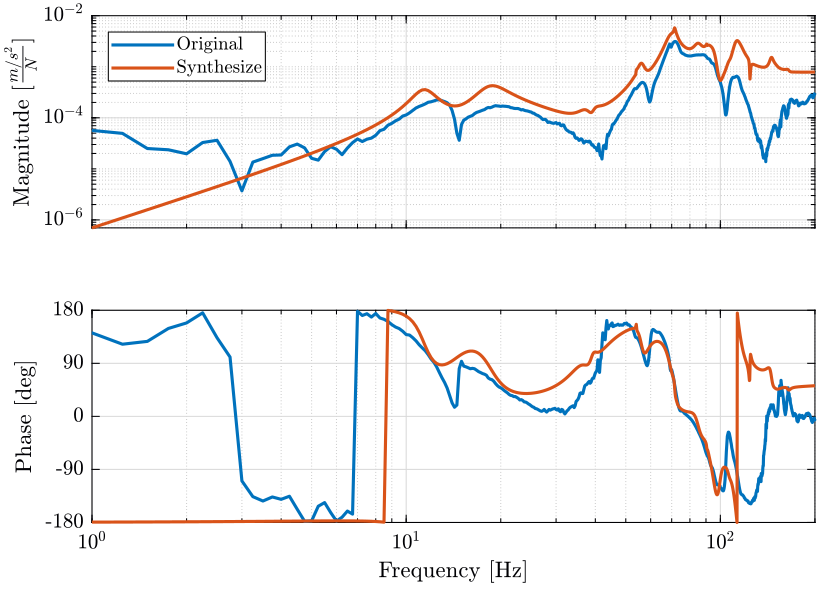
Figure 8: Comparison of the Original and Synthesize FRF matrix element
5.4 Synthesize FRF that has not yet been measured
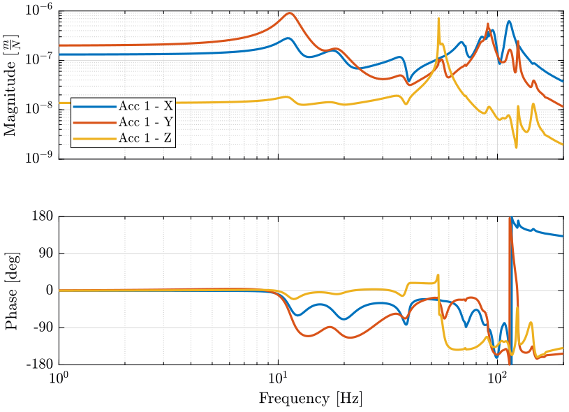
Figure 9: Synthesize FRF that has not been measured
6 Modal Complexity
A method of displaying modal complexity is by plotting the elements of the eigenvector on an Argand diagram (complex plane), such as the ones shown in figure 10.
To evaluate the complexity of the modes, we plot a polygon around the extremities of the individual vectors. The obtained area of this polygon is then compared with the area of the circle which is based on the length of the largest vector element. The resulting ratio is used as an indication of the complexity of the mode.
A mode with small complexity is shown on figure 10 whereas an highly complex mode is shown on figure 11. The complexity of all the modes are compared on figure 12.
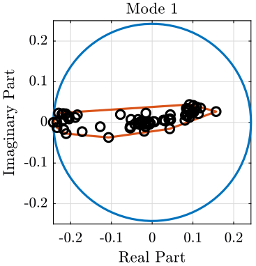
Figure 10: Modal Complexity of one mode with small complexity
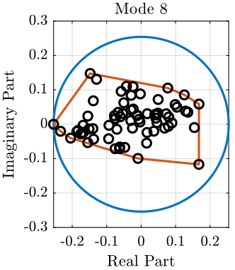
Figure 11: Modal Complexity of one higly complex mode
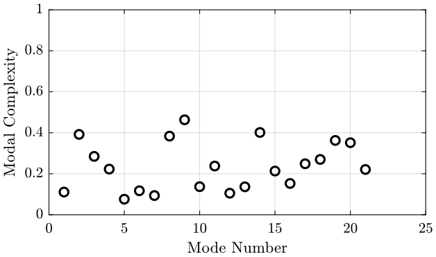
Figure 12: Modal complexity for each mode
7 Modal Assurance Criterion (MAC)
The MAC is calculated as the normalized scalar product of the two sets of vectors \(\{\psi_A\}\) and \(\{\psi_X\}\). The resulting scalars are arranged into the MAC matrix pastor12_modal_assur_criter:
\begin{equation} \text{MAC}(r, q) = \frac{\left| \{\psi_A\}_r^T \{\psi_X\}_q^* \right|^2}{\left( \{\psi_A\}_r^T \{\psi_A\}_r^* \right) \left( \{\psi_X\}_q^T \{\psi_X\}_q^* \right)} \end{equation}An equivalent formulation is:
\begin{equation} \text{MAC}(r, q) = \frac{\left| \sum_{j=1}^n \{\psi_A\}_j \{\psi_X\}_j^* \right|^2}{\left( \sum_{j=1}^n |\{\psi_A\}_j|^2 \right) \left( \sum_{j=1}^n |\{\psi_X\}_j|^2 \right)} \end{equation}The MAC takes value between 0 (representing no consistent correspondence) and 1 (representing a consistent correspondence).
We compute the autoMAC matrix that compares all the possible combinations of mode shape pairs for only one set of mode shapes. The result is shown on figure 13.
autoMAC = eye(size(eigen_vec_M, 2));

for r = 1:size(eigen_vec_M, 2)
  for q = r+1:size(eigen_vec_M, 2)
    autoMAC(r, q) = abs(eigen_vec_M(r, :)*eigen_vec_M(q, :)')^2/((eigen_vec_M(r, :)*eigen_vec_M(r, :)')*(eigen_vec_M(q, :)*eigen_vec_M(q, :)'));
    autoMAC(q, r) = autoMAC(r, q);
  end
end
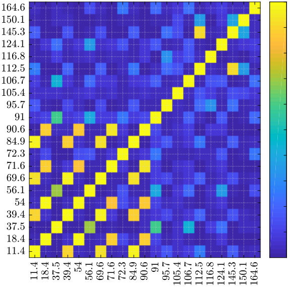
Figure 13: AutoMAC
8 From accelerometer coordinates to global coordinates for the mode shapes
8.1 Mathematical description
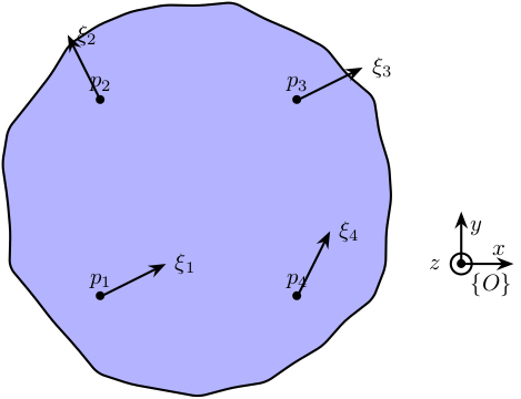
If we note \(\xi_i = \{ \xi_{i,x}\ \xi_{i,y}\ \xi_{i,z} \}^T\) the mode shape corresponding to the accelerometer \(i\).
From the figure above, we can write:
\begin{align*} \xi_1 &= \xi + \Omega p_1\\ \xi_2 &= \xi + \Omega p_2\\ \xi_3 &= \xi + \Omega p_3\\ \xi_4 &= \xi + \Omega p_4 \end{align*}With
\begin{equation} \Omega = \begin{bmatrix} 0 & -\Omega_z & \Omega_y \\ \Omega_z & 0 & -\Omega_x \\ -\Omega_y & \Omega_x & 0 \end{bmatrix} \end{equation}\(\xi\) and \(\Omega\) represent to mode shapes in translation and rotation of the solid expressed in the frame \(\{O\}\).
We can rearrange the equations in a matrix form, and then we obtain the mode shape of the solid in the wanted frame \(\{O\}\):
\begin{equation} \begin{bmatrix} \xi_x \\ \xi_y \\ \xi_z \\ \hline \Omega_x \\ \Omega_y \\ \Omega_z \end{bmatrix} = \left[\begin{array}{ccc|ccc} 1 & 0 & 0 & 0 & p_{1z} & -p_{1y} \\ 0 & 1 & 0 & -p_{1z} & 0 & p_{1x} \\ 0 & 0 & 1 & p_{1y} & -p_{1x} & 0 \\ \hline & \vdots & & & \vdots & \\ \hline 1 & 0 & 0 & 0 & p_{4z} & -p_{4y} \\ 0 & 1 & 0 & -p_{4z} & 0 & p_{4x} \\ 0 & 0 & 1 & p_{4y} & -p_{4x} & 0 \end{array}\right]^{-1} \begin{bmatrix} \xi_{1,x} \\ \xi_{1,y} \\ \xi_{1,z} \\\hline \vdots \\\hline \xi_{4,x} \\ \xi_{4,y} \\ \xi_{4,z} \end{bmatrix} \end{equation}This inversion is equivalent to a mean square problem.
8.2 Matlab Implementation
The obtained mode shapes matrix that gives the mode shapes of each solid bodies with respect to the fixed frame \(\{O\}\), mode_shapes_O, is an \(n \times p \times q\) with:
- \(n\) is the number of modes: 21
- \(p\) is the number of DOFs for each solid body: 6
- \(q\) is the number of solid bodies: 6
mode_shapes_O = zeros(mod_n, 6, length(solid_names));

for mod_i = 1:mod_n
  for solid_i = 1:length(solid_names)
    acc_i = solids.(solid_names{solid_i});

    Y = mode_shapes(mod_i, :, acc_i);
    Y = Y(:);

    A = zeros(3*length(acc_i), 6);
    for i = 1:length(acc_i)
      A(3*(i-1)+1:3*i, 1:3) = eye(3);

      A(3*(i-1)+1:3*i, 4:6) = [ 0              acc_pos(i, 3) -acc_pos(i, 2) ;
                               -acc_pos(i, 3)  0              acc_pos(i, 1) ;
                                acc_pos(i, 2) -acc_pos(i, 1)  0];
    end

    mode_shapes_O(mod_i, :, solid_i) = A\Y;
  end
end
We then rearrange the eigen vectors in another way: \[ \Psi_O = \begin{bmatrix} & & \\ \{\psi_1\} & \dots & \{\psi_N\} \\ & & \end{bmatrix}_{M \times N} \] with \[ \{\psi\}_r = \begin{Bmatrix} \psi_{1, x} & \psi_{1, y} & \psi_{1, z} & \psi_{1, \theta_x} & \psi_{1, \theta_y} & \psi_{1, \theta_z} & \psi_{2, x} & \dots & \psi_{6, \theta_z} \end{Bmatrix}^T \]
With \(M = 6 \times 6\) is the new number of DOFs and \(N=21\) is the number of modes.
eigen_vec_O = reshape(mode_shapes_O, [mod_n, 6*length(solid_names)]).';

eigen_vec_ext_O = [eigen_vec_O, conj(eigen_vec_O)];
8.3 FRF matrix synthesis
8.3.1 Mathematical description
The synthesize FRF matrix Hsyn_O is an \(n \times n \times q\) with:
- \(n\) is the number of DOFs of the considered 6 solid-bodies: \(6 \times 6 = 36\)
- \(q\) is the number of frequency points \(\omega_i\)
For each frequency point \(\omega_i\), the FRF matrix Hsyn_O is a \(n\times n\) matrix:
where \(D_i\) corresponds to the solid body number i, \(F_i\) is a force/torque applied on the solid body number i at the center of the frame \(\{O\}\).
As the mode shapes are expressed with respect to the frame \(\{O\}\), the obtain FRF matrix are the responses of the system from forces and torques applied to the solid bodies at the origin of \(\{O\}\) to the displacement of the solid bodies with respect to the frame \(\{O\}\).
8.3.2 Matlab Implementation
Hsyn_O = zeros(36, 36, 801);

for i = 1:length(freqs)
  Hsyn_O(:, :, i) = eigen_vec_ext_O*(inv(modal_a_ext_M)/(diag(j*2*pi*freqs(i) - diag(eigen_val_ext_M))))*eigen_vec_ext_O.';
end
Because the synthesize frequency response functions are representing the displacement response in \([m/N]\), we multiply each element of the FRF matrix by \((j \omega)^2\) in order to obtain the acceleration response in \([m/s^2/N]\).
for i = 1:size(Hsyn_O, 1)
  Hsyn_O(i, :, :) = -squeeze(Hsyn_O(i, :, :)).*(j*2*pi*freqs).^2;
end
8.3.3 TODO Test to have the original inputs
Hsyn_O = zeros(36, 3, 801);

for i = 1:length(freqs)
  Hsyn_O(:, :, i) = eigen_vec_ext_O*(inv(modal_a_ext_M)/(diag(j*2*pi*freqs(i) - diag(eigen_val_ext_M))))*eigen_vec_ext_M(10*3+1:11*3, :).';
end

for i = 1:size(Hsyn_O, 1)
  Hsyn_O(i, :, :) = -squeeze(Hsyn_O(i, :, :)).*(j*2*pi*freqs).^2;
end
8.4 TODO Verification
8.5 New FRFs
9 Some notes about constraining the number of degrees of freedom
We want to have the two eigen matrices.
They should have the same size \(n \times n\) where \(n\) is the number of modeshapes as well as the number of degrees of freedom. Thus, if we consider 21 modes, we should restrict our system to have only 21 DOFs.
Actually, we are measured 6 DOFs of 6 solids, thus we have 36 DOFs.
From the mode shapes animations, it seems that in the frequency range of interest, the two marbles can be considered as one solid. We thus have 5 solids and 30 DOFs.
In order to determine which DOF can be neglected, two solutions seems possible:
- compare the mode shapes
- compare the FRFs
The question is: in which base (frame) should be express the modes shapes and FRFs? Is it meaningful to compare mode shapes as they give no information about the amplitudes of vibration?
| Stage | Motion DOFs | Parasitic DOF | Total DOF | Description of DOF |
|---|---|---|---|---|
| Granite | 0 | 3 | 3 | |
| Ty | 1 | 2 | 3 | Ty, Rz |
| Ry | 1 | 2 | 3 | Ry, |
| Rz | 1 | 2 | 3 | Rz, Rx, Ry |
| Hexapod | 6 | 0 | 6 | Txyz, Rxyz |
| 9 | 9 | 18 |
10 Compare Mode Shapes
Let's say we want to see for the first mode which DOFs can be neglected. In order to do so, we should estimate the motion of each stage in particular directions. If we look at the z motion for instance, we will find that we cannot neglect that motion (because of the tilt causing z motion).
mode_i = 3;
dof_i = 6;

mode = eigen_vector_M(dof_i:6:end, mode_i);

figure;
hold on;
for i=1:length(mode)
  plot([0, real(mode(i))], [0, imag(mode(i))], '-', 'DisplayName', solid_names{i});
end
hold off;
legend();
figure;
subplot(2, 1, 1);
hold on;
for i=1:length(mode)
  plot(1, norm(mode(i)), 'o');
end
hold off;
ylabel('Amplitude');

subplot(2, 1, 2);
hold on;
for i=1:length(mode)
  plot(1, 180/pi*angle(mode(i)), 'o', 'DisplayName', solid_names{i});
end
hold off;
ylim([-180, 180]); yticks([-180:90:180]);
ylabel('Phase [deg]');
legend();
test = mode_shapes_O(10, 1, :)/norm(squeeze(mode_shapes_O(10, 1, :)));
test = mode_shapes_O(10, 2, :)/norm(squeeze(mode_shapes_O(10, 2, :)));
11 TODO Mode shapes expressed in a frame at the CoM of the solid bodies
Maybe the mass-normalized eigen vectors can only be obtained for undamped systems (real eigen values and vectors).
11.1 Modes shapes transformation
First, we load the position of the Center of Mass of each solid body with respect to the point of interest.
model_com = table2array(readtable('mat/model_solidworks_com.txt', 'ReadVariableNames', false));
Then, we reshape the data.
model_com = reshape(model_com , [3, 6]);
Now we convert the mode shapes expressed in the DOF of the accelerometers to the DoF of each solid body (translations and rotations) with respect to their own CoM.
mode_shapes_CoM = zeros(mod_n, 6, length(solid_names));

for mod_i = 1:mod_n
  for solid_i = 1:length(solid_names)
    acc_i = solids.(solid_names{solid_i});

    Y = mode_shapes(mod_i, :, acc_i);
    Y = Y(:);

    A = zeros(3*length(acc_i), 6);
    for i = 1:length(acc_i)
      acc_pos_com = acc_pos(i, :).' - model_com(:, i);

      A(3*(i-1)+1:3*i, 1:3) = eye(3);
      A(3*(i-1)+1:3*i, 4:6) = [ 0               acc_pos_com(3) -acc_pos_com(2) ;
                               -acc_pos_com(3)  0               acc_pos_com(1) ;
                                acc_pos_com(2) -acc_pos_com(1)  0];
    end

    mode_shapes_CoM(mod_i, :, solid_i) = A\Y;
  end
end
We then rearrange the eigen vectors in another way: \[ \Psi_{\text{CoM}} = \begin{bmatrix} & & \\ \{\psi_1\} & \dots & \{\psi_N\} \\ & & \end{bmatrix}_{M \times N} \] with \[ \{\psi\}_r = \begin{Bmatrix} \psi_{1, x} & \psi_{1, y} & \psi_{1, z} & \psi_{1, \theta_x} & \psi_{1, \theta_y} & \psi_{1, \theta_z} & \psi_{2, x} & \dots & \psi_{6, \theta_z} \end{Bmatrix}^T \]
With \(M = 6 \times 6\) is the new number of DOFs and \(N=21\) is the number of modes.
Each eigen vector is normalized.
eigen_vec_CoM = reshape(mode_shapes_CoM, [mod_n, 6*length(solid_names)]).';
% eigen_vec_CoM = eigen_vec_CoM./vecnorm(eigen_vec_CoM);
eigen_vec_ext_CoM = [eigen_vec_CoM, conj(eigen_vec_CoM)];
11.2 Mass matrix from solidworks model
sed '/Mass = /!d' mat/1_granite_bot.txt | sed 's/^\s*\t*Mass = //' | sed 's/\([0-9.]*\) kilograms\r/\1/' >  mat/model_solidworks_mass.txt
sed '/Mass = /!d' mat/2_granite_top.txt | sed 's/^\s*\t*Mass = //' | sed 's/\([0-9.]*\) kilograms\r/\1/' >> mat/model_solidworks_mass.txt
sed '/Mass = /!d' mat/3_ty.txt          | sed 's/^\s*\t*Mass = //' | sed 's/\([0-9.]*\) kilograms\r/\1/' >> mat/model_solidworks_mass.txt
sed '/Mass = /!d' mat/4_ry.txt          | sed 's/^\s*\t*Mass = //' | sed 's/\([0-9.]*\) kilograms\r/\1/' >> mat/model_solidworks_mass.txt
sed '/Mass = /!d' mat/5_rz.txt          | sed 's/^\s*\t*Mass = //' | sed 's/\([0-9.]*\) kilograms\r/\1/' >> mat/model_solidworks_mass.txt
sed '/Mass = /!d' mat/6_hexa.txt        | sed 's/^\s*\t*Mass = //' | sed 's/\([0-9.]*\) kilograms\r/\1/' >> mat/model_solidworks_mass.txt
sed '/I[xyz][xyz]/!d' mat/1_granite_bot.txt | sed 's/^\s*\t*//' | sed 's/I[xyz][xyz] = //g' | sed $'s/\r//' >  mat/model_solidworks_inertia.txt
sed '/I[xyz][xyz]/!d' mat/2_granite_top.txt | sed 's/^\s*\t*//' | sed 's/I[xyz][xyz] = //g' | sed $'s/\r//' >> mat/model_solidworks_inertia.txt
sed '/I[xyz][xyz]/!d' mat/3_ty.txt          | sed 's/^\s*\t*//' | sed 's/I[xyz][xyz] = //g' | sed $'s/\r//' >> mat/model_solidworks_inertia.txt
sed '/I[xyz][xyz]/!d' mat/4_ry.txt          | sed 's/^\s*\t*//' | sed 's/I[xyz][xyz] = //g' | sed $'s/\r//' >> mat/model_solidworks_inertia.txt
sed '/I[xyz][xyz]/!d' mat/5_rz.txt          | sed 's/^\s*\t*//' | sed 's/I[xyz][xyz] = //g' | sed $'s/\r//' >> mat/model_solidworks_inertia.txt
sed '/I[xyz][xyz]/!d' mat/6_hexa.txt        | sed 's/^\s*\t*//' | sed 's/I[xyz][xyz] = //g' | sed $'s/\r//' >> mat/model_solidworks_inertia.txt
model_mass = table2array(readtable('mat/model_solidworks_mass.txt', 'ReadVariableNames', false));
model_inertia = table2array(readtable('mat/model_solidworks_inertia.txt', 'ReadVariableNames', false));
\[ M = \begin{bmatrix} M_1 & & & & & \\ & M_2 & & & & \\ & & M_3 & & & \\ & & & M_4 & & \\ & & & & M_5 & \\ & & & & & M_6 \\ \end{bmatrix}, \text{ with } M_i = \begin{bmatrix} m_i & & & & & \\ & m_i & & & & \\ & & m_i & & & \\ & & & I_{i,xx} & I_{i,yx} & I_{i,zx} \\ & & & I_{i,xy} & I_{i,yy} & I_{i,zy} \\ & & & I_{i,xz} & I_{i,yz} & I_{i,zz} \\ \end{bmatrix} \]
M = zeros(6*6, 6*6);

for i = 1:6
  M((i-1)*6+1:i*6, (i-1)*6+1:i*6) = blkdiag(model_mass(i)*eye(3), model_inertia((i-1)*3+1:i*3, 1:3));
end
11.3 Mass-normalized Eigen Vectors
To do so, it seems that we need to know the mass matrix \([M]\). Then: \[ \{\phi\}_r = \frac{1}{\sqrt{m_r}} \{\psi\}_r \text{ where } m_r = \{\psi\}_r^T [M] \{\psi\}_r \]
Mass-normalized eigen vectors are very important for the synthesis and spatial model extraction.
Mass Matrix could be estimated from the SolidWorks model.
We compute the modal masses that will be used for normalization.
mr = zeros(size(eigen_vector_matrix_CoM, 2), 1);

for i = 1:length(mr)
  mr(i) = real(eigen_vector_matrix_CoM(:, i).' * M * eigen_vector_matrix_CoM(:, i));
end
figure;
plot(freqs_m, mr, 'ko');
xlabel('Mode Frequency [Hz]'); ylabel('Modal mass [kg]');
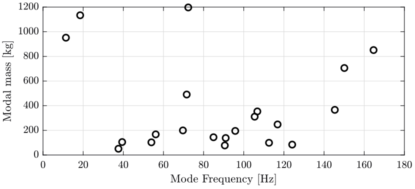
Figure 15: Modal masses
And finally, we compute the mass-normalized eigen vectors.
eigen_vector_mass_CoM = zeros(size(eigen_vector_matrix_CoM));

for i = 1:size(eigen_vector_matrix_CoM, 2)
  eigen_vector_mass_CoM(:, i) = 1/sqrt(mr(i)) * eigen_vector_matrix_CoM(:, i);
end
Verification that \[ [\Phi]^T [M] [\Phi] = [I] \]
eigen_vector_matrix_CoM.'*M*eigen_vector_matrix_CoM
eigen_vector_mass_CoM*M*eigen_vector_mass_CoM.'
Other test for normalized eigen vectors
eigen_vector_mass_CoM = (eigen_vector_matrix_CoM.'*diag(diag(M))*eigen_vector_matrix_CoM)^(-0.5) * eigen_vector_matrix_CoM';
eigen_vector_mass_CoM = eigen_vector_mass_CoM.';
11.4 Full Response Model from modal model (synthesis)
In general, the form of response model with which we are concerned is an FRF matrix whose order is dictated by the number of coordinates \(n\) included in the test. Also, as explained, it is normal in practice to measured and to analyze just a subset of the FRF matrix but rather to measure the full FRF matrix. Usually one column or one row with a few additional elements are measured.
Thus, if we are to construct an acceptable response model, it will be necessary to synthesize those elements which have not been directly measured. However, in principle, this need present no major problem as it is possible to compute the full FRF matrix from a modal model using:
\begin{equation} [H]_{n\times n} = [\Phi]_{n\times m} [\lambda_r^2 - \omega^2]_{m\times m}^{-1} [\Phi]_{m\times n}^T \end{equation}\(\{\Phi\}\) is a mass-normalized eigen vector.
FRF_matrix_CoM = zeros(size(eigen_vector_mass_CoM, 1), size(eigen_vector_mass_CoM, 1), length(freqs));

for i = 1:length(freqs)
  FRF_matrix_CoM(:, :, i) = eigen_vector_mass_CoM*inv(eigen_value_M^2 - (2*pi*freqs(i)*eye(size(eigen_value_M, 1)))^2)*eigen_vector_mass_CoM.';
end
exc_dir = 3;
meas_mass = 6;
meas_dir = 3;

figure;
hold on;
plot(freqs, abs(squeeze(FRF_matrix_CoM((meas_mass-1)*6 + meas_dir, 6*2+exc_dir, :))));
plot(freqs, abs(squeeze(FRFs_CoM((meas_mass-1)*6 + meas_dir, exc_dir, :))));
hold off;
set(gca, 'XScale', 'log'); set(gca, 'YScale', 'log');
xlabel('Frequency [Hz]'); ylabel('Amplitude');
xlim([1, 200]);
FRF_matrix = zeros(size(eigen_vector_mass, 1), size(eigen_vector_mass, 1), length(freqs));

for i = 1:length(freqs)
  FRF_matrix(:, :, i) = eigen_vector_mass*inv(eigen_value_M - (freqs(i)*eye(size(eigen_value_M, 1)))^2)*eigen_vector_mass.';
end
figure;
hold on;
plot(freqs, abs(squeeze(FRFs_O(1, 1, :))));
plot(freqs, abs(squeeze(FRF_matrix(1, 1, :))));
hold off;
set(gca, 'XScale', 'log'); set(gca, 'YScale', 'log');
xlabel('Frequency [Hz]'); ylabel('Amplitude');
xlim([1, 200]);
12 TODO Residues
Bibliography
- [pastor12_modal_assur_criter] Miroslav Pastor, Michal Binda & Tom\'a\vs Har\vcarik, Modal Assurance Criterion, Procedia Engineering, 48(nil), 543-548 (2012). link. doi.