Static Measurements
Table of Contents
1 Ty Stage
All the files (data and Matlab scripts) are accessible here.
1.1 Notes
- 5530: Straightness Plot: Yz
- Filename:
r:\home\PDMU\PEL\Measurement_library\ID31\ID31_u_station\TY\12_12_2018\linear deviation _tyz_401_points.txt - Acquisition date: 09/01/2019 13:49:42
- Current date: 08/03/2019 08:46:35
- Measurement Type: STRAIGHTNESS vertical
- Travel Mode: Bidirectional
- Number of Target Positions: 401
- Number of total data pairs: 2406
- Number of total data runs:6
- Position Value Units: millimeters
- Error Value Units: micrometers
| Environmental Data | Min | Max | Avg |
|---|---|---|---|
| Air Temp (C) | 024,57 | 024,61 | 024,59 |
| Air Prs (mm) | 742,56 | 743,29 | 742,83 |
| Air Hmd (%) | 024,00 | 024,00 | 024,00 |
| MT1 Temp (C) | 020,00 | ||
| MT2 Temp (C) | 024,40 | 024,44 | 024,42 |
| MT3 Temp (C) | 024,32 | 024,36 | 024,34 |
In a very schematic way, the measurement is explained on figure 1. The positioning error \(d\) is measure as a function of \(x\). Because the measurement is done in a static way, the dynamics of the station (represented by the mass-spring-damper system on the schematic) does not play a role in the measure.
The obtained data corresponds to the guiding errors.

Figure 1: Schematic of the measurement
1.2 Data Pre-processing
sed 's/\t/ /g;s/\,/./g' "mat/linear_deviation_tyz_401_points.txt" > data/data_tyz.txt
head "mat/data_tyz.txt"
| Run | Pos | TargetValue | ErrorValue |
|---|---|---|---|
| 1 | 1 | -4.5E+00 | 7.5377892E+00 |
| 1 | 2 | -4.4775E+00 | 7.5422246E+00 |
| 1 | 3 | -4.455E+00 | 7.5655617E+00 |
| 1 | 4 | -4.4325E+00 | 7.5149518E+00 |
| 1 | 5 | -4.41E+00 | 7.4886377E+00 |
| 1 | 6 | -4.3875E+00 | 7.437007E+00 |
| 1 | 7 | -4.365E+00 | 7.4449354E+00 |
| 1 | 8 | -4.3425E+00 | 7.3937387E+00 |
| 1 | 9 | -4.32E+00 | 7.3287468E+00 |
1.3 Matlab - Data Import
filename = 'mat/data_tyz.txt';
fileID = fopen(filename);
data = cell2mat(textscan(fileID,'%f  %f  %f  %f', 'collectoutput', 1,'headerlines',1));
fclose(fileID);
1.4 Data - Plot
First, we plot the straightness error as a function of the position (figure 2).
figure;
hold on;
for i=1:data(end, 1)
  plot(data(data(:, 1) == i, 3), data(data(:, 1) == i, 4), '-k');
end
hold off;
xlabel('Target Value [mm]'); ylabel('Error Value [$\mu m$]');
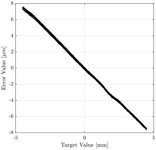
Figure 2: Time domain Data
Then, we compute mean value of each position, and we remove this mean value from the data. The results are shown on figure 3.
mean_pos = zeros(sum(data(:, 1)==1), 1);
for i=1:sum(data(:, 1)==1)
  mean_pos(i) = mean(data(data(:, 2)==i, 4));
end
figure;
hold on;
for i=1:data(end, 1)
  filt = data(:, 1) == i;
  plot(data(filt, 3), data(filt, 4) - mean_pos, '-k');
end
hold off;
xlabel('Target Value [mm]'); ylabel('Error Value [$\mu m$]');
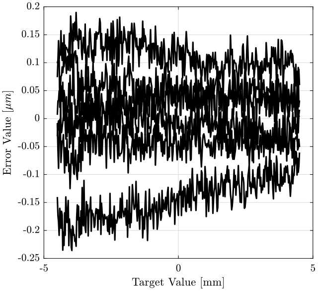
Figure 3: caption
1.5 Translate to time domain
We here make the assumptions that, during a scan with the translation stage, the Z motion of the translation stage will follow the guiding error measured.
We then create a time vector \(t\) from 0 to 1 second that corresponds to a typical scan, and we plot the guiding error as a function of the time on figure 4.
t = linspace(0, 1, length(data(data(:, 1)==1, 4)));
figure;
hold on;
plot(t, data(data(:, 1) == 1, 4) - mean_pos, '-k');
hold off;
xlabel('Time [s]'); ylabel('Error Value [um]');
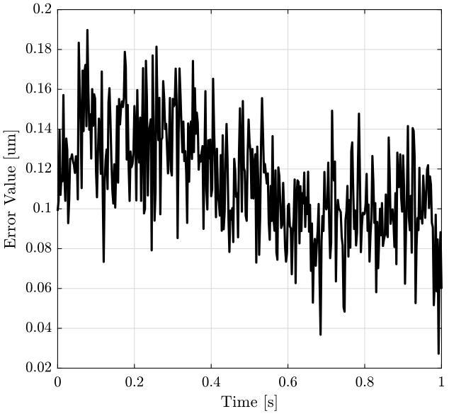
Figure 4: caption
1.6 Compute the PSD
We first compute some parameters that will be used for the PSD computation.
dt = t(2)-t(1);

Fs = 1/dt; % [Hz]

win = hanning(ceil(1*Fs));
We remove the mean position from the data.
x = data(data(:, 1) == 1, 4) - mean_pos;
And finally, we compute the power spectral density of the displacement obtained in the time domain.
The result is shown on figure 5.
[pxx, f] = pwelch(x, win, [], [], Fs);

pxx_t = zeros(length(pxx), data(end, 1));

for i=1:data(end, 1)
  x = data(data(:, 1) == i, 4) - mean_pos;
  [pxx, f] = pwelch(x, win, [], [], Fs);
  pxx_t(:, i) = pxx;
end
figure;
hold on;
plot(f, sqrt(mean(pxx_t, 2)), 'k-');
hold off;
xlabel('Frequency (Hz)');
ylabel('Amplitude Spectral Density $\left[\frac{m}{\sqrt{Hz}}\right]$');
set(gca, 'XScale', 'log'); set(gca, 'YScale', 'log');
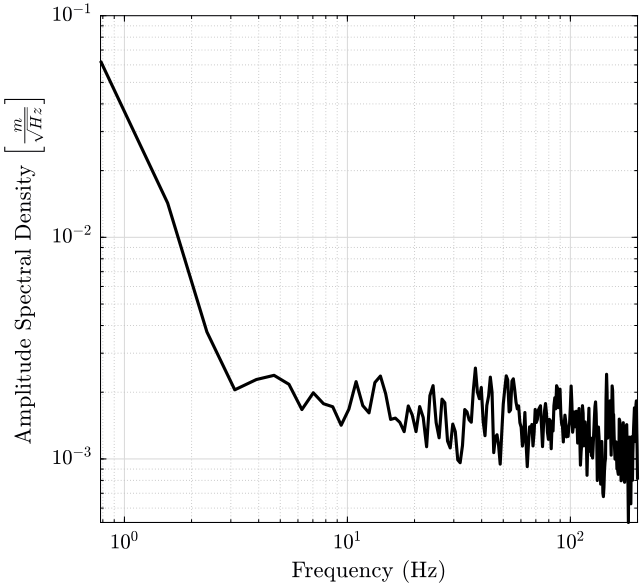
Figure 5: PSD of the Z motion when scanning with Ty at 1Hz