Finite Element Model with Simscape
Table of Contents
1 Amplified Piezoelectric Actuator - 3D elements
The idea here is to:
- export a FEM of an amplified piezoelectric actuator from Ansys to Matlab
- import it into a Simscape model
- compare the obtained dynamics
- add 10kg mass on top of the actuator and identify the dynamics
- compare with results from Ansys where 10kg are directly added to the FEM
1.1 Import Mass Matrix, Stiffness Matrix, and Interface Nodes Coordinates
We first extract the stiffness and mass matrices.
K = extractMatrix('piezo_amplified_3d_K.txt');
M = extractMatrix('piezo_amplified_3d_M.txt');
Then, we extract the coordinates of the interface nodes.
[int_xyz, int_i, n_xyz, n_i, nodes] = extractNodes('piezo_amplified_3d.txt');
| Total number of Nodes | 168959 |
| Number of interface Nodes | 13 |
| Number of Modes | 30 |
| Size of M and K matrices | 108 |
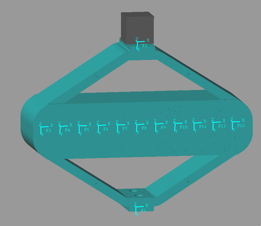
Figure 1: Interface Nodes for the Amplified Piezo Actuator
| Node i | Node Number | x [m] | y [m] | z [m] |
|---|---|---|---|---|
| 1.0 | 168947.0 | 0.0 | 0.03 | 0.0 |
| 2.0 | 168949.0 | 0.0 | -0.03 | 0.0 |
| 3.0 | 168950.0 | -0.035 | 0.0 | 0.0 |
| 4.0 | 168951.0 | -0.028 | 0.0 | 0.0 |
| 5.0 | 168952.0 | -0.021 | 0.0 | 0.0 |
| 6.0 | 168953.0 | -0.014 | 0.0 | 0.0 |
| 7.0 | 168954.0 | -0.007 | 0.0 | 0.0 |
| 8.0 | 168955.0 | 0.0 | 0.0 | 0.0 |
| 9.0 | 168956.0 | 0.007 | 0.0 | 0.0 |
| 10.0 | 168957.0 | 0.014 | 0.0 | 0.0 |
| 11.0 | 168958.0 | 0.021 | 0.0 | 0.0 |
| 12.0 | 168959.0 | 0.035 | 0.0 | 0.0 |
| 13.0 | 168960.0 | 0.028 | 0.0 | 0.0 |
| 300000000.0 | -30000.0 | 8000.0 | -200.0 | -30.0 | -60000.0 | 20000000.0 | -4000.0 | 500.0 | 8 |
| -30000.0 | 100000000.0 | 400.0 | 30.0 | 200.0 | -1 | 4000.0 | -8000000.0 | 800.0 | 7 |
| 8000.0 | 400.0 | 50000000.0 | -800000.0 | -300.0 | -40.0 | 300.0 | 100.0 | 5000000.0 | 40000.0 |
| -200.0 | 30.0 | -800000.0 | 20000.0 | 5 | 1 | -10.0 | -2 | -40000.0 | -300.0 |
| -30.0 | 200.0 | -300.0 | 5 | 40000.0 | 0.3 | -4 | -10.0 | 40.0 | 0.4 |
| -60000.0 | -1 | -40.0 | 1 | 0.3 | 3000.0 | 7000.0 | 0.8 | -1 | 0.0003 |
| 20000000.0 | 4000.0 | 300.0 | -10.0 | -4 | 7000.0 | 300000000.0 | 20000.0 | 3000.0 | 80.0 |
| -4000.0 | -8000000.0 | 100.0 | -2 | -10.0 | 0.8 | 20000.0 | 100000000.0 | -4000.0 | -100.0 |
| 500.0 | 800.0 | 5000000.0 | -40000.0 | 40.0 | -1 | 3000.0 | -4000.0 | 50000000.0 | 800000.0 |
| 8 | 7 | 40000.0 | -300.0 | 0.4 | 0.0003 | 80.0 | -100.0 | 800000.0 | 20000.0 |
| 0.03 | 2e-06 | -2e-07 | 1e-08 | 2e-08 | 0.0002 | -0.001 | 2e-07 | -8e-08 | -9e-10 |
| 2e-06 | 0.02 | -5e-07 | 7e-09 | 3e-08 | 2e-08 | -3e-07 | 0.0003 | -1e-08 | 1e-10 |
| -2e-07 | -5e-07 | 0.02 | -9e-05 | 4e-09 | -1e-08 | 2e-07 | -2e-08 | -0.0006 | -5e-06 |
| 1e-08 | 7e-09 | -9e-05 | 1e-06 | 6e-11 | 4e-10 | -1e-09 | 3e-11 | 5e-06 | 3e-08 |
| 2e-08 | 3e-08 | 4e-09 | 6e-11 | 1e-06 | 2e-10 | -2e-09 | 2e-10 | -7e-09 | -4e-11 |
| 0.0002 | 2e-08 | -1e-08 | 4e-10 | 2e-10 | 2e-06 | -2e-06 | -1e-09 | -7e-10 | -9e-12 |
| -0.001 | -3e-07 | 2e-07 | -1e-09 | -2e-09 | -2e-06 | 0.03 | -2e-06 | -1e-07 | -5e-09 |
| 2e-07 | 0.0003 | -2e-08 | 3e-11 | 2e-10 | -1e-09 | -2e-06 | 0.02 | -8e-07 | -1e-08 |
| -8e-08 | -1e-08 | -0.0006 | 5e-06 | -7e-09 | -7e-10 | -1e-07 | -8e-07 | 0.02 | 9e-05 |
| -9e-10 | 1e-10 | -5e-06 | 3e-08 | -4e-11 | -9e-12 | -5e-09 | -1e-08 | 9e-05 | 1e-06 |
Using K, M and int_xyz, we can use the Reduced Order Flexible Solid simscape block.
1.2 Identification of the Dynamics
The flexible element is imported using the Reduced Order Flexible Solid simscape block.
To model the actuator, an Internal Force block is added between the nodes 3 and 12.
A Relative Motion Sensor block is added between the nodes 1 and 2 to measure the displacement and the amplified piezo.
One mass is fixed at one end of the piezo-electric stack actuator, the other end is fixed to the world frame.
We first set the mass to be zero.
m = 0;
The dynamics is identified from the applied force to the measured relative displacement.
%% Name of the Simulink File
mdl = 'piezo_amplified_3d';

%% Input/Output definition
clear io; io_i = 1;
io(io_i) = linio([mdl, '/F'], 1, 'openinput');  io_i = io_i + 1;
io(io_i) = linio([mdl, '/y'], 1, 'openoutput'); io_i = io_i + 1;

Gh = linearize(mdl, io);
Then, we add 10Kg of mass:
m = 10;
And the dynamics is identified.
The two identified dynamics are compared in Figure 2.
%% Name of the Simulink File
mdl = 'piezo_amplified_3d';

%% Input/Output definition
clear io; io_i = 1;
io(io_i) = linio([mdl, '/F'], 1, 'openinput');  io_i = io_i + 1;
io(io_i) = linio([mdl, '/y'], 1, 'openoutput'); io_i = io_i + 1;

Ghm = linearize(mdl, io);
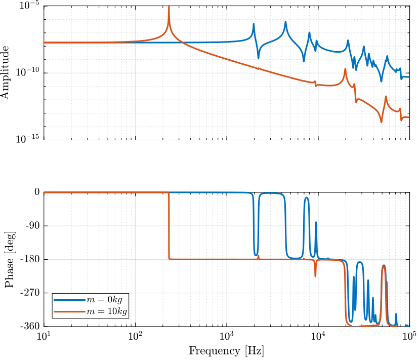
Figure 2: Dynamics from \(F\) to \(d\) without a payload and with a 10kg payload
1.3 Comparison with Ansys
Let’s import the results from an Harmonic response analysis in Ansys.
Gresp0 = readtable('FEA_HarmResponse_00kg.txt');
Gresp10 = readtable('FEA_HarmResponse_10kg.txt');
The obtained dynamics from the Simscape model and from the Ansys analysis are compare in Figure 3.
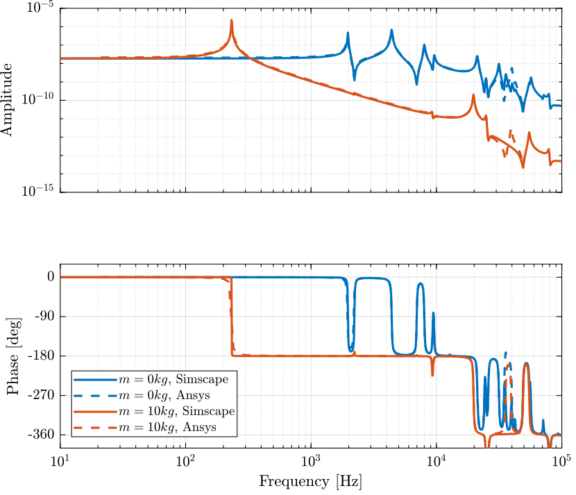
Figure 3: Comparison of the obtained dynamics using Simscape with the harmonic response analysis using Ansys
1.4 Force Sensor
The dynamics is identified from internal forces applied between nodes 3 and 11 to the relative displacement of nodes 11 and 13.
The obtained dynamics is shown in Figure 4.
m = 0;
%% Name of the Simulink File
mdl = 'piezo_amplified_3d';

%% Input/Output definition
clear io; io_i = 1;
io(io_i) = linio([mdl, '/Fa'], 1, 'openinput');  io_i = io_i + 1;
io(io_i) = linio([mdl, '/Fs'], 1, 'openoutput'); io_i = io_i + 1;

Gf = linearize(mdl, io);
m = 10;
%% Name of the Simulink File
mdl = 'piezo_amplified_3d';

%% Input/Output definition
clear io; io_i = 1;
io(io_i) = linio([mdl, '/Fa'], 1, 'openinput');  io_i = io_i + 1;
io(io_i) = linio([mdl, '/Fs'], 1, 'openoutput'); io_i = io_i + 1;

Gfm = linearize(mdl, io);

Figure 4: Dynamics from \(F\) to \(F_m\) for \(m=0\) and \(m = 10kg\)
1.5 Distributed Actuator
m = 0;
The dynamics is identified from the applied force to the measured relative displacement.
%% Name of the Simulink File
mdl = 'piezo_amplified_3d_distri';

%% Input/Output definition
clear io; io_i = 1;
io(io_i) = linio([mdl, '/F'], 1, 'openinput');  io_i = io_i + 1;
io(io_i) = linio([mdl, '/y'], 1, 'openoutput'); io_i = io_i + 1;

Gd = linearize(mdl, io);
Then, we add 10Kg of mass:
m = 10;
And the dynamics is identified.
%% Name of the Simulink File
mdl = 'piezo_amplified_3d_distri';

%% Input/Output definition
clear io; io_i = 1;
io(io_i) = linio([mdl, '/F'], 1, 'openinput');  io_i = io_i + 1;
io(io_i) = linio([mdl, '/y'], 1, 'openoutput'); io_i = io_i + 1;

Gdm = linearize(mdl, io);
1.6 Distributed Actuator and Force Sensor
m = 0;
%% Name of the Simulink File
mdl = 'piezo_amplified_3d_distri_act_sens';

%% Input/Output definition
clear io; io_i = 1;
io(io_i) = linio([mdl, '/F'], 1, 'openinput');  io_i = io_i + 1;
io(io_i) = linio([mdl, '/Fm'], 1, 'openoutput'); io_i = io_i + 1;

Gfd = linearize(mdl, io);
m = 10;
%% Name of the Simulink File
mdl = 'piezo_amplified_3d_distri_act_sens';

%% Input/Output definition
clear io; io_i = 1;
io(io_i) = linio([mdl, '/F'], 1, 'openinput');  io_i = io_i + 1;
io(io_i) = linio([mdl, '/Fm'], 1, 'openoutput'); io_i = io_i + 1;

Gfdm = linearize(mdl, io);
2 Integral Force Feedback with Amplified Piezo
2.1 Import Mass Matrix, Stiffness Matrix, and Interface Nodes Coordinates
We first extract the stiffness and mass matrices.
K = extractMatrix('piezo_amplified_IFF_K.txt');
M = extractMatrix('piezo_amplified_IFF_M.txt');
Then, we extract the coordinates of the interface nodes.
[int_xyz, int_i, n_xyz, n_i, nodes] = extractNodes('piezo_amplified_IFF.txt');
2.2 IFF Plant
The transfer function from the force actuator to the force sensor is identified and shown in Figure 5.
Kiff = tf(0);
m = 0;
%% Name of the Simulink File
mdl = 'piezo_amplified_IFF';

%% Input/Output definition
clear io; io_i = 1;
io(io_i) = linio([mdl, '/Kiff'], 1, 'openinput');  io_i = io_i + 1;
io(io_i) = linio([mdl, '/G'],    1, 'openoutput'); io_i = io_i + 1;

Gf = linearize(mdl, io);
m = 10;
Gfm = linearize(mdl, io);
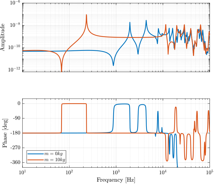
Figure 5: IFF Plant
2.3 IFF controller
The controller is defined and the loop gain is shown in Figure 6.
Kiff = -1e12/s;
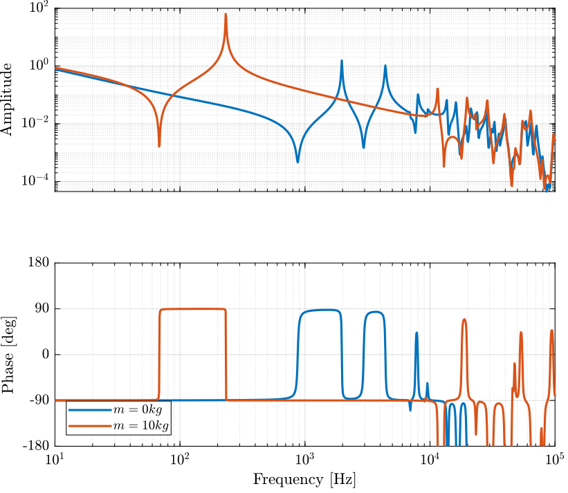
Figure 6: IFF Loop Gain
2.4 Closed Loop System
m = 10;
Kiff = -1e12/s;
%% Name of the Simulink File
mdl = 'piezo_amplified_IFF';

%% Input/Output definition
clear io; io_i = 1;
io(io_i) = linio([mdl, '/Dw'], 1, 'openinput');  io_i = io_i + 1;
io(io_i) = linio([mdl, '/F'],  1, 'openinput');  io_i = io_i + 1;
io(io_i) = linio([mdl, '/Fd'], 1, 'openinput');  io_i = io_i + 1;
io(io_i) = linio([mdl, '/d'],  1, 'openoutput'); io_i = io_i + 1;
io(io_i) = linio([mdl, '/G'],  1, 'output'); io_i = io_i + 1;

Giff = linearize(mdl, io);
Giff.InputName  = {'w', 'f', 'F'};
Giff.OutputName  = {'x1', 'Fs'};
Kiff = tf(0);
G = linearize(mdl, io);
G.InputName  = {'w', 'f', 'F'};
G.OutputName  = {'x1', 'Fs'};
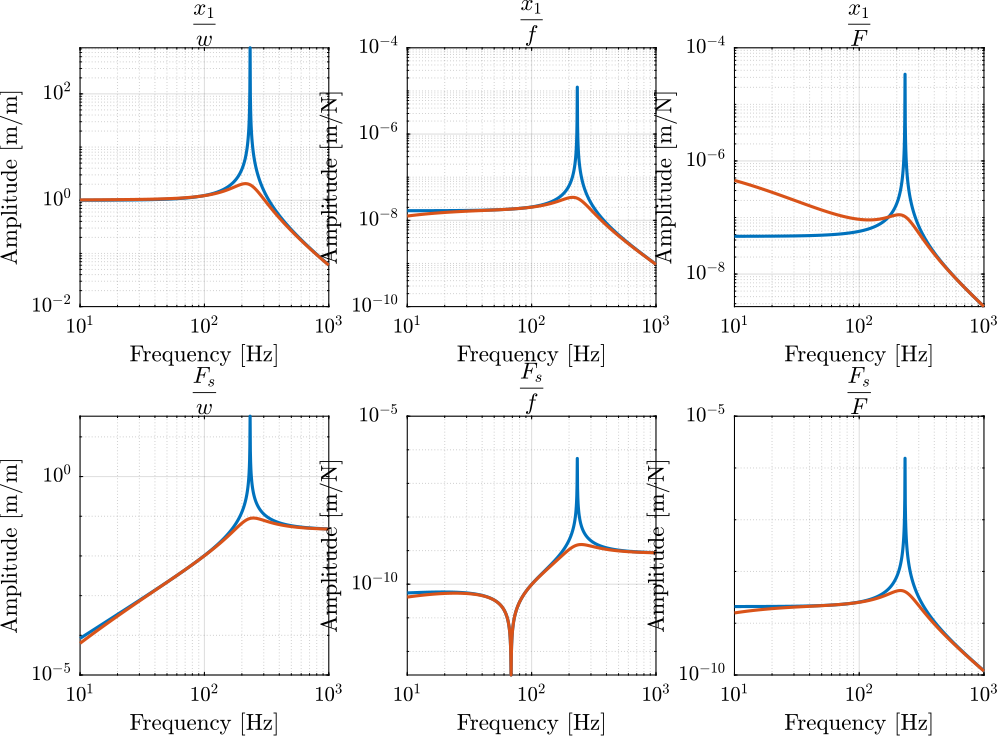
Figure 7: OL and CL transfer functions
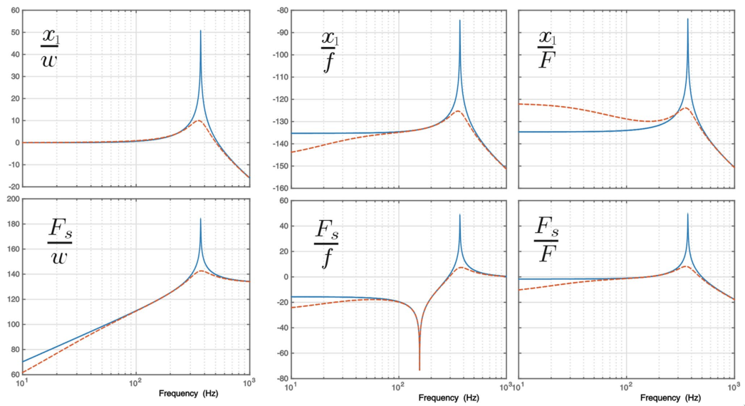
Figure 8: Results obtained in souleille18_concep_activ_mount_space_applic