Robust and Optimal Sensor Fusion - Matlab Computation
Table of Contents
In this document, the optimal and robust design of complementary filters is studied.
Two sensors are considered with both different noise characteristics and dynamical uncertainties represented by multiplicative input uncertainty.
- Section 3: the \(\mathcal{H}_2\) synthesis is used to design complementary filters such that the RMS value of the super sensor’s noise is minimized
- Section 4: the \(\mathcal{H}_\infty\) synthesis is used to design complementary filters such that the super sensor’s uncertainty is bonded to acceptable values
- Section 5: the mixed \(\mathcal{H}_2/\mathcal{H}_\infty\) synthesis is used to both limit the super sensor’s uncertainty and to lower the RMS value of the super sensor’s noise
1 Sensor Description
In Figure 1 is shown a schematic of a sensor model that is used in the following study. In this example, the measured quantity \(x\) is the velocity of an object.
| Notation | Meaning | Unit |
|---|---|---|
| \(x\) | Physical measured quantity | \([m/s]\) |
| \(\tilde{n}_i\) | White noise with unitary PSD | |
| \(n_i\) | Shaped noise | \([m/s]\) |
| \(v_i\) | Sensor output measurement | \([V]\) |
| \(\hat{x}_i\) | Estimate of \(x\) from the sensor | \([m/s]\) |
| Notation | Meaning | Unit |
|---|---|---|
| \(\hat{G}_i\) | Nominal Sensor Dynamics | \([\frac{V}{m/s}]\) |
| \(W_i\) | Weight representing the size of the uncertainty at each frequency | |
| \(\Delta_i\) | Any complex perturbation such that \(\vert\vert\Delta_i\vert\vert_\infty < 1\) | |
| \(N_i\) | Weight representing the sensor noise | \([m/s]\) |

Figure 1: Sensor Model
1.1 Sensor Dynamics
Let’s consider two sensors measuring the velocity of an object.
The first sensor is an accelerometer. Its nominal dynamics \(\hat{G}_1(s)\) is defined below.
m_acc = 0.01; % Inertial Mass [kg]
c_acc = 5;    % Damping [N/(m/s)]
k_acc = 1e5;  % Stiffness [N/m]
g_acc = 1e5;  % Gain [V/m]

G1 = g_acc*m_acc*s/(m_acc*s^2 + c_acc*s + k_acc); % Accelerometer Plant [V/(m/s)]
The second sensor is a displacement sensor, its nominal dynamics \(\hat{G}_2(s)\) is defined below.
w_pos = 2*pi*2e3; % Measurement Banwdith [rad/s]
g_pos = 1e4; % Gain [V/m]

G2 = g_pos/s/(1 + s/w_pos); % Position Sensor Plant [V/(m/s)]
These nominal dynamics are also taken as the model of the sensor dynamics. The true sensor dynamics has some uncertainty associated to it and described in section 1.2.
Both sensor dynamics in \([\frac{V}{m/s}]\) are shown in Figure 2.
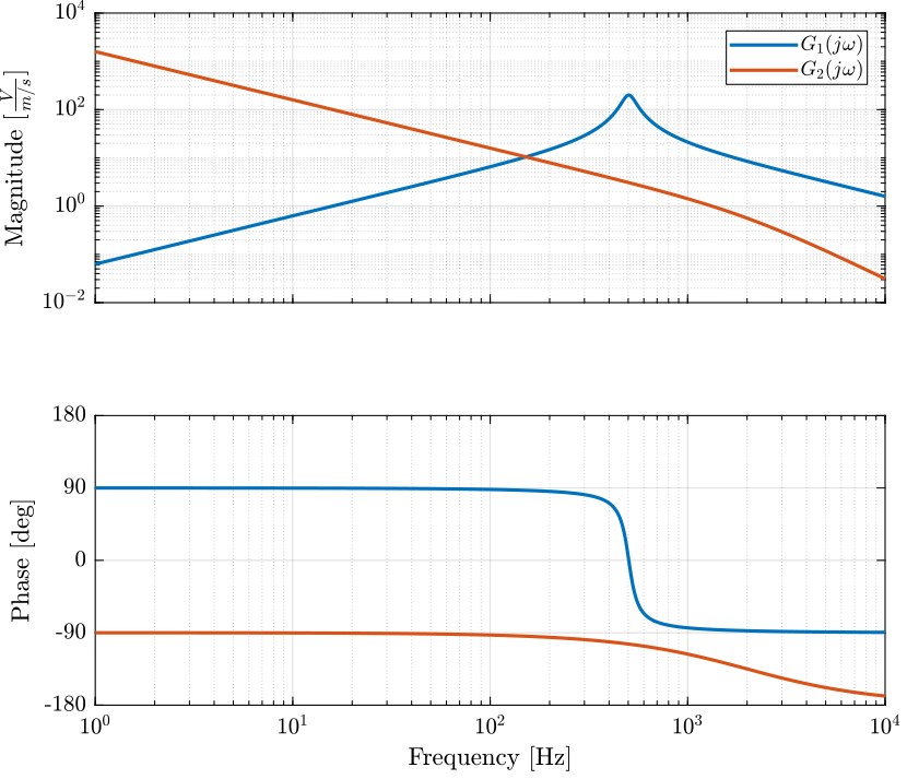
Figure 2: Sensor nominal dynamics from the velocity of the object to the output voltage
1.2 Sensor Model Uncertainty
The uncertainty on the sensor dynamics is described by multiplicative uncertainty (Figure 1).
The true sensor dynamics \(G_i(s)\) is then described by \eqref{eq:sensor_dynamics_uncertainty}.
\begin{equation} G_i(s) = \hat{G}_i(s) \left( 1 + W_i(s) \Delta_i(s) \right); \quad |\Delta_i(j\omega)| < 1 \forall \omega \label{eq:sensor_dynamics_uncertainty} \end{equation}The weights \(W_i(s)\) representing the dynamical uncertainty are defined below and their magnitude is shown in Figure 3.
W1 = createWeight('n', 2, 'w0', 2*pi*3,   'G0', 2, 'G1', 0.1,     'Gc', 1) * ...
     createWeight('n', 2, 'w0', 2*pi*1e3, 'G0', 1, 'G1', 4/0.1, 'Gc', 1/0.1);

W2 = createWeight('n', 2, 'w0', 2*pi*1e2, 'G0', 0.05, 'G1', 4, 'Gc', 1);
The bode plot of the sensors nominal dynamics as well as their defined dynamical spread are shown in Figure 4.
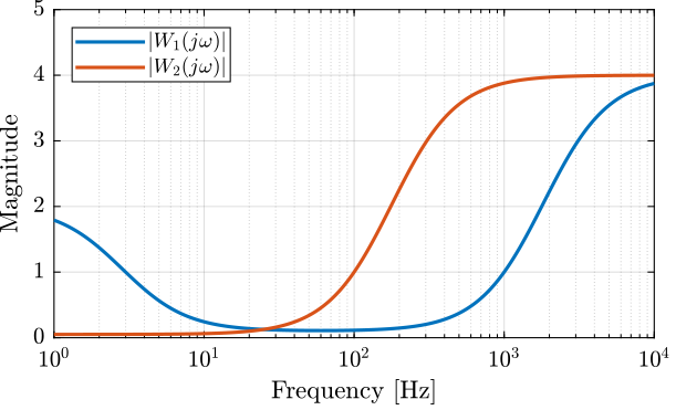
Figure 3: Magnitude of the multiplicative uncertainty weights \(|W_i(j\omega)|\)
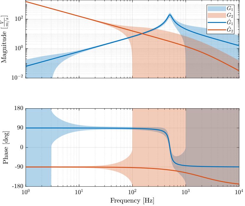
Figure 4: Nominal Sensor Dynamics \(\hat{G}_i\) (solid lines) as well as the spread of the dynamical uncertainty (background color)
1.3 Sensor Noise
The noise of the sensors \(n_i\) are modelled by shaping a white noise with unitary PSD \(\tilde{n}_i\) \eqref{eq:unitary_noise_psd} with a LTI transfer function \(N_i(s)\) (Figure 1).
\begin{equation} \Phi_{\tilde{n}_i}(\omega) = 1 \label{eq:unitary_noise_psd} \end{equation}The Power Spectral Density of the sensor noise \(\Phi_{n_i}(\omega)\) is then computed using \eqref{eq:sensor_noise_shaping} and expressed in \([\frac{(m/s)^2}{Hz}]\).
\begin{equation} \Phi_{n_i}(\omega) = \left| N_i(j\omega) \right|^2 \Phi_{\tilde{n}_i}(\omega) \label{eq:sensor_noise_shaping} \end{equation}The weights \(N_1\) and \(N_2\) representing the amplitude spectral density of the sensor noises are defined below and shown in Figure 5.
omegac = 0.15*2*pi; G0 = 1e-1; Ginf = 1e-6;
N1 = (Ginf*s/omegac + G0)/(s/omegac + 1)/(1 + s/2/pi/1e4);

omegac = 1000*2*pi; G0 = 1e-6; Ginf = 1e-3;
N2 = (Ginf*s/omegac + G0)/(s/omegac + 1)/(1 + s/2/pi/1e4);
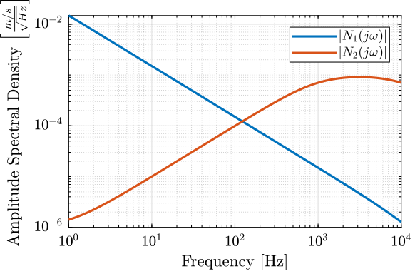
Figure 5: Amplitude spectral density of the sensors \(\sqrt{\Phi_{n_i}(\omega)} = |N_i(j\omega)|\)
1.4 Save Model
All the dynamical systems representing the sensors are saved for further use.
save('./mat/model.mat', 'freqs', 'G1', 'G2', 'N2', 'N1', 'W2', 'W1');
2 Introduction to Sensor Fusion
2.1 Sensor Fusion Architecture
The two sensors presented in Section 1 are now merged together using complementary filters \(H_1(s)\) and \(H_2(s)\) to form a super sensor (Figure 6).

Figure 6: Sensor Fusion Architecture
The complementary property of \(H_1(s)\) and \(H_2(s)\) means that the sum of their transfer function is equal to \(1\) \eqref{eq:complementary_property}.
\begin{equation} H_1(s) + H_2(s) = 1 \label{eq:complementary_property} \end{equation}The super sensor estimate \(\hat{x}\) is given by \eqref{eq:super_sensor_estimate}.
\begin{equation} \hat{x} = \left( H_1 \hat{G}_1^{-1} G_1 + H_2 \hat{G}_2^{-1} G_2 \right) x + \left( H_1 \hat{G}_1^{-1} G_1 N_1 \right) \tilde{n}_1 + \left( H_2 \hat{G}_2^{-1} G_2 N_2 \right) \tilde{n}_2 \label{eq:super_sensor_estimate} \end{equation}2.2 Super Sensor Noise
If we first suppose that the models of the sensors \(\hat{G}_i\) are very close to the true sensor dynamics \(G_i\) \eqref{eq:good_dynamical_model}, we have that the super sensor estimate \(\hat{x}\) is equals to the measured quantity \(x\) plus the noise of the two sensors filtered out by the complementary filters \eqref{eq:estimate_perfect_models}.
\begin{equation} \hat{G}_i^{-1}(s) G_i(s) \approx 1 \label{eq:good_dynamical_model} \end{equation} \begin{equation} \hat{x} = x + \underbrace{\left( H_1 N_1 \right) \tilde{n}_1 + \left( H_2 N_2 \right) \tilde{n}_2}_{n} \label{eq:estimate_perfect_models} \end{equation}As the noise of both sensors are considered to be uncorrelated, the PSD of the super sensor noise is computed as follow:
\begin{equation} \Phi_n(\omega) = \left| H_1(j\omega) N_1(j\omega) \right|^2 + \left| H_2(j\omega) N_2(j\omega) \right|^2 \label{eq:super_sensor_psd_noise} \end{equation}And the Root Mean Square (RMS) value of the super sensor noise \(\sigma_n\) is given by Equation \eqref{eq:super_sensor_rms_noise}.
\begin{equation} \sigma_n = \sqrt{\int_0^\infty \Phi_n(\omega) d\omega} \label{eq:super_sensor_rms_noise} \end{equation}2.3 Super Sensor Dynamical Uncertainty
If we consider some dynamical uncertainty (the true system dynamics \(G_i\) not being perfectly equal to our model \(\hat{G}_i\)) that we model by the use of multiplicative uncertainty (Figure 7), the super sensor dynamics is then equals to:
\begin{equation} \begin{aligned} \frac{\hat{x}}{x} &= \Big( H_1 \hat{G}_1^{-1} \hat{G}_1 (1 + W_1 \Delta_1) + H_2 \hat{G}_2^{-1} \hat{G}_2 (1 + W_2 \Delta_2) \Big) \\ &= \Big( H_1 (1 + W_1 \Delta_1) + H_2 (1 + W_2 \Delta_2) \Big) \\ &= \left( 1 + H_1 W_1 \Delta_1 + H_2 W_2 \Delta_2 \right), \quad \|\Delta_i\|_\infty<1 \end{aligned} \end{equation}
Figure 7: Sensor Model including Dynamical Uncertainty
The uncertainty set of the transfer function from \(\hat{x}\) to \(x\) at frequency \(\omega\) is bounded in the complex plane by a circle centered on 1 and with a radius equal to \(|W_1(j\omega) H_1(j\omega)| + |W_2(j\omega) H_2(j\omega)|\) as shown in Figure 8.

Figure 8: Super Sensor model uncertainty displayed in the complex plane
3 Optimal Super Sensor Noise: \(\mathcal{H}_2\) Synthesis
In this section, the complementary filters \(H_1(s)\) and \(H_2(s)\) are designed in order to minimize the RMS value of super sensor noise \(\sigma_n\).

Figure 9: Optimal Sensor Fusion Architecture
The RMS value of the super sensor noise is (neglecting the model uncertainty):
\begin{equation} \begin{aligned} \sigma_{n} &= \sqrt{\int_0^\infty |H_1(j\omega) N_1(j\omega)|^2 + |H_2(j\omega) N_2(j\omega)|^2 d\omega} \\ &= \left\| \begin{matrix} H_1 N_1 \\ H_2 N_2 \end{matrix} \right\|_2 \end{aligned} \end{equation}The goal is to design \(H_1(s)\) and \(H_2(s)\) such that \(H_1(s) + H_2(s) = 1\) (complementary property) and such that \(\left\| \begin{matrix} H_1 N_1 \\ H_2 N_2 \end{matrix} \right\|_2\) is minimized (minimized RMS value of the super sensor noise). This is done using the \(\mathcal{H}_2\) synthesis in Section 3.1.
3.1 \(\mathcal{H}_2\) Synthesis
Consider the generalized plant \(P_{\mathcal{H}_2}\) shown in Figure 10 and described by Equation \eqref{eq:H2_generalized_plant}.

Figure 10: Architecture used for \(\mathcal{H}_\infty\) synthesis of complementary filters
Applying the \(\mathcal{H}_2\) synthesis on \(P_{\mathcal{H}_2}\) will generate a filter \(H_2(s)\) such that the \(\mathcal{H}_2\) norm from \(w\) to \((z_1,z_2)\) which is actually equals to \(\sigma_n\) by defining \(H_1(s) = 1 - H_2(s)\):
\begin{equation} \left\| \begin{matrix} z_1/w \\ z_2/w \end{matrix} \right\|_2 = \left\| \begin{matrix} N_1 (1 - H_2) \\ N_2 H_2 \end{matrix} \right\|_2 = \sigma_n \quad \text{with} \quad H_1(s) = 1 - H_2(s) \end{equation}We then have that the \(\mathcal{H}_2\) synthesis applied on \(P_{\mathcal{H}_2}\) generates two complementary filters \(H_1(s)\) and \(H_2(s)\) such that the RMS value of super sensor noise is minimized.
The generalized plant \(P_{\mathcal{H}_2}\) is defined below
PH2 = [N1 -N1;
       0   N2;
       1   0];
The \(\mathcal{H}_2\) synthesis using the h2syn command
[H2, ~, gamma] = h2syn(PH2, 1, 1);
Finally, \(H_1(s)\) is defined as follows
H1 = 1 - H2;
The obtained complementary filters are shown in Figure 11.
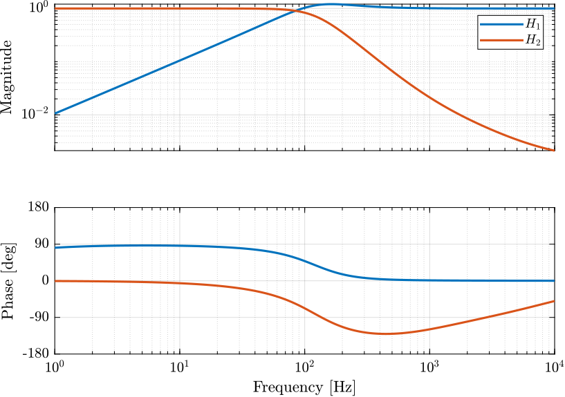
Figure 11: Obtained complementary filters using the \(\mathcal{H}_2\) Synthesis
3.2 Super Sensor Noise
The Power Spectral Density of the individual sensors’ noise \(\Phi_{n_1}, \Phi_{n_2}\) and of the super sensor noise \(\Phi_{n_{\mathcal{H}_2}}\) are computed below and shown in Figure 12.
PSD_S1 = abs(squeeze(freqresp(N1,    freqs, 'Hz'))).^2;
PSD_S2 = abs(squeeze(freqresp(N2,    freqs, 'Hz'))).^2;
PSD_H2 = abs(squeeze(freqresp(N1*H1, freqs, 'Hz'))).^2 + ...
         abs(squeeze(freqresp(N2*H2, freqs, 'Hz'))).^2;
The corresponding Cumulative Power Spectrum \(\Gamma_{n_1}\), \(\Gamma_{n_2}\) and \(\Gamma_{n_{\mathcal{H}_2}}\) (cumulative integration of the PSD \eqref{eq:CPS_definition}) are computed below and shown in Figure 13.
CPS_S1 = cumtrapz(freqs, PSD_S1);
CPS_S2 = cumtrapz(freqs, PSD_S2);
CPS_H2 = cumtrapz(freqs, PSD_H2);
The RMS value of the individual sensors and of the super sensor are listed in Table 3.
| RMS value \([m/s]\) | |
|---|---|
| \(\sigma_{n_1}\) | 0.015 |
| \(\sigma_{n_2}\) | 0.080 |
| \(\sigma_{n_{\mathcal{H}_2}}\) | 0.003 |
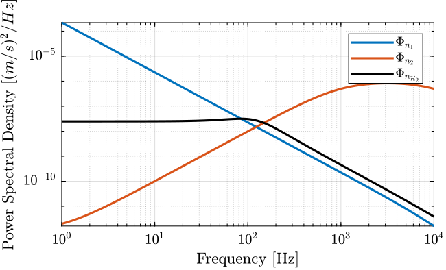
Figure 12: Power Spectral Density of the estimated \(\hat{x}\) using the two sensors alone and using the optimally fused signal
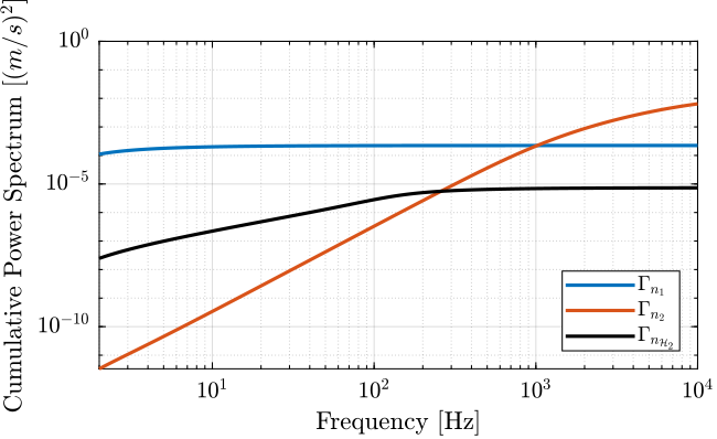
Figure 13: Cumulative Power Spectrum of individual sensors and super sensor using the \(\mathcal{H}_2\) synthesis
A time domain simulation is now performed. The measured velocity \(x\) is set to be a sweep sine with an amplitude of \(0.1\ [m/s]\). The velocity estimates from the two sensors and from the super sensors are shown in Figure 14. The resulting noises are displayed in Figure 15.
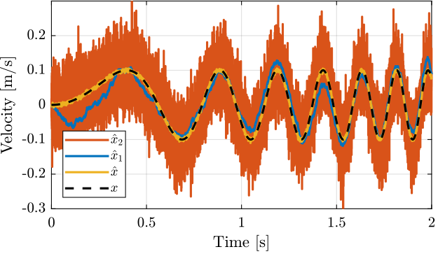
Figure 14: Noise of individual sensors and noise of the super sensor
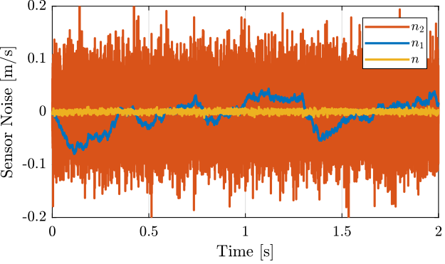
Figure 15: Noise of the two sensors \(n_1, n_2\) and noise of the super sensor \(n\)
3.3 Discrepancy between sensor dynamics and model
If we consider sensor dynamical uncertainty as explained in Section 1.2, we can compute what would be the super sensor dynamical uncertainty when using the complementary filters obtained using the \(\mathcal{H}_2\) Synthesis.
The super sensor dynamical uncertainty is shown in Figure 16.
It is shown that the phase uncertainty is not bounded between 100Hz and 200Hz. As a result the super sensor signal can not be used for feedback applications about 100Hz.
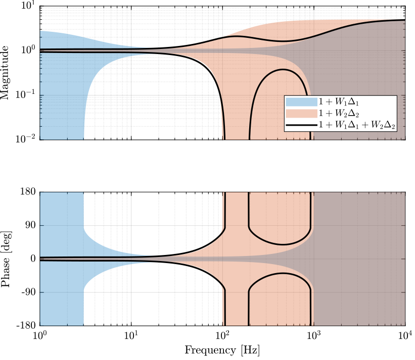
Figure 16: Super sensor dynamical uncertainty when using the \(\mathcal{H}_2\) Synthesis
4 Robust Sensor Fusion: \(\mathcal{H}_\infty\) Synthesis
We initially considered perfectly known sensor dynamics so that it can be perfectly inverted.
We now take into account the fact that the sensor dynamics is only partially known. To do so, we model the uncertainty that we have on the sensor dynamics by multiplicative input uncertainty as shown in Figure 17.

Figure 17: Sensor fusion architecture with sensor dynamics uncertainty
As explained in Section 1.2, at each frequency \(\omega\), the dynamical uncertainty of the super sensor can be represented in the complex plane by a circle with a radius equals to \(|H_1(j\omega) W_1(j\omega)| + |H_2(j\omega) W_2(j\omega)|\) and centered on 1.
In order to specify a wanted upper bound on the dynamical uncertainty, a weight \(W_u(s)\) is used where \(1/|W_u(j\omega)|\) represents the maximum allowed radius of the uncertainty circle corresponding to the super sensor dynamics at a frequency \(\omega\) \eqref{eq:upper_bound_uncertainty}.
\begin{align} & |H_1(j\omega) W_1(j\omega)| + |H_2(j\omega) W_2(j\omega)| < \frac{1}{|W_u(j\omega)|}, \quad \forall \omega \label{eq:upper_bound_uncertainty} \\ \Leftrightarrow & |H_1(j\omega) W_1(j\omega) W_u(j\omega)| + |H_2(j\omega) W_2(j\omega) W_u(j\omega)| < 1, \quad \forall\omega \label{eq:upper_bound_uncertainty_bis} \end{align}\(|W_u(j\omega)|\) is also linked to the gain uncertainty \(\Delta G\) \eqref{eq:gain_uncertainty_bound} and phase uncertainty \(\Delta\phi\) \eqref{eq:phase_uncertainty_bound} of the super sensor.
\begin{align} \Delta G (\omega) &\le \frac{1}{|W_u(j\omega)|}, \quad \forall\omega \label{eq:gain_uncertainty_bound} \\ \Delta \phi (\omega) &\le \arcsin\left(\frac{1}{|W_u(j\omega)|}\right), \quad \forall\omega \label{eq:phase_uncertainty_bound} \end{align}The choice of \(W_u\) is presented in Section 4.1.
Condition \eqref{eq:upper_bound_uncertainty_bis} can almost be represented by \eqref{eq:hinf_norm_uncertainty} (within a factor \(\sqrt{2}\)).
\begin{equation} \left\| \begin{matrix} H_1(s) W_1(s) W_u(s) \\ H_2(s) W_2(s) W_u(s) \end{matrix} \right\|_\infty < 1 \label{eq:hinf_norm_uncertainty} \end{equation}The objective is to design \(H_1(s)\) and \(H_2(s)\) such that \(H_1(s) + H_2(s) = 1\) (complementary property) and such that \eqref{eq:hinf_norm_uncertainty} is verified (bounded dynamical uncertainty).
This is done using the \(\mathcal{H}_\infty\) synthesis in Section 4.2.
4.1 Weighting Function used to bound the super sensor uncertainty
\(W_u(s)\) is defined such that the super sensor phase uncertainty is less than 10 degrees below 100Hz \eqref{eq:phase_uncertainy_bound_low_freq} and is less than 180 degrees below 400Hz \eqref{eq:phase_uncertainty_max}.
\begin{align} \frac{1}{|W_u(j\omega)|} &< \sin\left(10 \frac{\pi}{180}\right), \quad \omega < 100\,\text{Hz} \label{eq:phase_uncertainy_bound_low_freq} \\ \frac{1}{|W_u(j 2 \pi 400)|} &< 1 \label{eq:phase_uncertainty_max} \end{align}The uncertainty bounds of the two individual sensor as well as the wanted maximum uncertainty bounds of the super sensor are shown in Figure 18.
Dphi = 10; % [deg]

Wu = createWeight('n', 2, 'w0', 2*pi*4e2, 'G0', 1/sin(Dphi*pi/180), 'G1', 1/4, 'Gc', 1);

Figure 18: Uncertainty region of the two sensors as well as the wanted maximum uncertainty of the super sensor (dashed lines)
4.2 \(\mathcal{H}_\infty\) Synthesis
The generalized plant \(P_{\mathcal{H}_\infty}\) used for the \(\mathcal{H}_\infty\) Synthesis of the complementary filters is shown in Figure 19 and is described by Equation \eqref{eq:Hinf_generalized_plant}.

Figure 19: Architecture used for \(\mathcal{H}_\infty\) synthesis of complementary filters
The generalized plant is defined below.
P = [Wu*W1 -Wu*W1;
     0      Wu*W2;
     1      0];
And the \(\mathcal{H}_\infty\) synthesis is performed using the hinfsyn command.
H2 = hinfsyn(P, 1, 1,'TOLGAM', 0.001, 'DISPLAY', 'on');
Test bounds:  0.7071 <=  gamma  <=  1.291

  gamma        X>=0        Y>=0       rho(XY)<1    p/f
9.554e-01     0.0e+00     0.0e+00     3.529e-16     p
8.219e-01     0.0e+00     0.0e+00     5.204e-16     p
7.624e-01     3.8e-17     0.0e+00     1.955e-15     p
7.342e-01     0.0e+00     0.0e+00     5.612e-16     p
7.205e-01     0.0e+00     0.0e+00     7.184e-16     p
7.138e-01     0.0e+00     0.0e+00     0.000e+00     p
7.104e-01     4.1e-16     0.0e+00     6.749e-15     p
7.088e-01     0.0e+00     0.0e+00     2.794e-15     p
7.079e-01     0.0e+00     0.0e+00     6.503e-16     p
7.075e-01     0.0e+00     0.0e+00     4.302e-15     p

Best performance (actual): 0.7071
The \(\mathcal{H}_\infty\) is successful as the \(\mathcal{H}_\infty\) norm of the “closed loop” transfer function from \((w)\) to \((z_1,\ z_2)\) is less than one.
\(H_1(s)\) is then defined as the complementary of \(H_2(s)\).
H1 = 1 - H2;
The obtained complementary filters as well as the wanted upper bounds are shown in Figure 20.
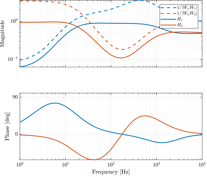
Figure 20: Obtained complementary filters using the \(\mathcal{H}_\infty\) Synthesis
4.3 Super sensor uncertainty
The super sensor dynamical uncertainty is displayed in Figure 21. It is confirmed that the super sensor dynamical uncertainty is less than the maximum allowed uncertainty defined by the norm of \(W_u(s)\).
The frequency band where the super sensor has small dynamical uncertainty is larger than for the individual sensor.
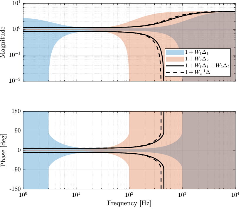
Figure 21: Super sensor dynamical uncertainty (solid curve) when using the \(\mathcal{H}_\infty\) Synthesis
4.4 Super sensor noise
We now compute the obtain Power Spectral Density of the super sensor’s noise (Figure 22).
The obtained RMS of the super sensor noise in the \(\mathcal{H}_2\) and \(\mathcal{H}_\infty\) case are shown in Table 4. As expected, the super sensor obtained from the \(\mathcal{H}_\infty\) synthesis is much noisier than the super sensor obtained from the \(\mathcal{H}_2\) synthesis.
PSD_S2   = abs(squeeze(freqresp(N2,    freqs, 'Hz'))).^2;
PSD_S1   = abs(squeeze(freqresp(N1,    freqs, 'Hz'))).^2;
PSD_Hinf = abs(squeeze(freqresp(N1*H1, freqs, 'Hz'))).^2 + ...
           abs(squeeze(freqresp(N2*H2, freqs, 'Hz'))).^2;
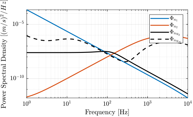
Figure 22: Power Spectral Density of the estimated \(\hat{x}\) using the two sensors alone and using the
| RMS [m/s] | |
|---|---|
| Optimal: \(\mathcal{H}_2\) | 0.0027 |
| Robust: \(\mathcal{H}_\infty\) | 0.041 |
4.5 Conclusion
Using the \(\mathcal{H}_\infty\) synthesis, the dynamical uncertainty of the super sensor can be bounded to acceptable values.
However, the RMS of the super sensor noise is not optimized as it was the case with the \(\mathcal{H}_2\) synthesis
5 Optimal and Robust Sensor Fusion: Mixed \(\mathcal{H}_2/\mathcal{H}_\infty\) Synthesis

Figure 23: Sensor fusion architecture with sensor dynamics uncertainty
The goal is to design complementary filters such that:
- the maximum uncertainty of the super sensor is bounded
- the RMS value of the super sensor noise is minimized
To do so, we can use the Mixed \(\mathcal{H}_2\) / \(\mathcal{H}_\infty\) Synthesis.
The Matlab function for that is h2hinfsyn (doc).
5.1 Mixed \(\mathcal{H}_2\) / \(\mathcal{H}_\infty\) Synthesis
The synthesis architecture that is used here is shown in Figure 24.
The controller \(K\) is synthesized such that it:
- Keeps the \(\mathcal{H}_\infty\) norm \(G\) of the transfer function from \(w\) to \(z_\infty\) bellow some specified value
- Keeps the \(\mathcal{H}_2\) norm \(H\) of the transfer function from \(w\) to \(z_2\) bellow some specified value
- Minimizes a trade-off criterion of the form \(W_1 G^2 + W_2 H^2\) where \(W_1\) and \(W_2\) are specified values

Figure 24: Mixed \(\mathcal{H}_2/\mathcal{H}_\infty\) Synthesis
Here, we define \(P\) such that:
\begin{align*} \left\| \frac{z_\infty}{w} \right\|_\infty &= \left\| \begin{matrix}W_1(s) H_1(s) \\ W_2(s) H_2(s)\end{matrix} \right\|_\infty \\ \left\| \frac{z_2}{w} \right\|_2 &= \left\| \begin{matrix}N_1(s) H_1(s) \\ N_2(s) H_2(s)\end{matrix} \right\|_2 \end{align*}Then:
- we specify the maximum value for the \(\mathcal{H}_\infty\) norm between \(w\) and \(z_\infty\) to be \(1\)
- we don’t specify any maximum value for the \(\mathcal{H}_2\) norm between \(w\) and \(z_2\)
- we choose \(W_1 = 0\) and \(W_2 = 1\) such that the objective is to minimize the \(\mathcal{H}_2\) norm between \(w\) and \(z_2\)
The synthesis objective is to have: \[ \left\| \frac{z_\infty}{w} \right\|_\infty = \left\| \begin{matrix}W_1(s) H_1(s) \\ W_2(s) H_2(s)\end{matrix} \right\|_\infty < 1 \] and to minimize: \[ \left\| \frac{z_2}{w} \right\|_2 = \left\| \begin{matrix}N_1(s) H_1(s) \\ N_2(s) H_2(s)\end{matrix} \right\|_2 \] which is what we wanted.
We define the generalized plant that will be used for the mixed synthesis.
W1u = ss(W2*Wu); W2u = ss(W1*Wu); % Weight on the uncertainty
W1n = ss(N2); W2n = ss(N1); % Weight on the noise

P = [W1u -W1u;
     0    W2u;
     W1n -W1n;
     0    W2n;
     1    0];
The mixed \(\mathcal{H}_2/\mathcal{H}_\infty\) synthesis is performed below.
Nmeas = 1; Ncon = 1; Nz2 = 2;

[H1, ~, normz, ~] = h2hinfsyn(P, Nmeas, Ncon, Nz2, [0, 1], 'HINFMAX', 1, 'H2MAX', Inf, 'DKMAX', 100, 'TOL', 0.01, 'DISPLAY', 'on');

H2 = 1 - H1;
The obtained complementary filters are shown in Figure 25.

Figure 25: Obtained complementary filters after mixed \(\mathcal{H}_2/\mathcal{H}_\infty\) synthesis
5.2 Obtained Super Sensor’s noise
The PSD and CPS of the super sensor’s noise are shown in Figure 26 and Figure 27 respectively.
PSD_S2     = abs(squeeze(freqresp(N2, freqs, 'Hz'))).^2;
PSD_S1     = abs(squeeze(freqresp(N1, freqs, 'Hz'))).^2;
PSD_H2Hinf = abs(squeeze(freqresp(N1*H1, freqs, 'Hz'))).^2+abs(squeeze(freqresp(N2*H2, freqs, 'Hz'))).^2;

CPS_S2     = cumtrapz(freqs, PSD_S2);
CPS_S1     = cumtrapz(freqs, PSD_S1);
CPS_H2Hinf = cumtrapz(freqs, PSD_H2Hinf);

Figure 26: Power Spectral Density of the Super Sensor obtained with the mixed \(\mathcal{H}_2/\mathcal{H}_\infty\) synthesis

Figure 27: Cumulative Power Spectrum of the Super Sensor obtained with the mixed \(\mathcal{H}_2/\mathcal{H}_\infty\) synthesis
5.3 Obtained Super Sensor’s Uncertainty
The uncertainty on the super sensor’s dynamics is shown in Figure
5.4 Comparison Hinf H2 H2/Hinf
H2_filters      = load('./mat/H2_filters.mat',      'H2', 'H1');
Hinf_filters    = load('./mat/Hinf_filters.mat',    'H2', 'H1');
H2_Hinf_filters = load('./mat/H2_Hinf_filters.mat', 'H2', 'H1');
PSD_H2 = abs(squeeze(freqresp(N2*H2_filters.H2, freqs, 'Hz'))).^2+abs(squeeze(freqresp(N1*H2_filters.H1, freqs, 'Hz'))).^2;
CPS_H2 = cumtrapz(freqs, PSD_H2);

PSD_Hinf = abs(squeeze(freqresp(N2*Hinf_filters.H2, freqs, 'Hz'))).^2+abs(squeeze(freqresp(N1*Hinf_filters.H1, freqs, 'Hz'))).^2;
CPS_Hinf = cumtrapz(freqs, PSD_Hinf);

PSD_H2Hinf = abs(squeeze(freqresp(N2*H2_Hinf_filters.H2, freqs, 'Hz'))).^2+abs(squeeze(freqresp(N1*H2_Hinf_filters.H1, freqs, 'Hz'))).^2;
CPS_H2Hinf = cumtrapz(freqs, PSD_H2Hinf);
| RMS [m/s] | |
|---|---|
| Optimal: \(\mathcal{H}_2\) | 0.0012 |
| Robust: \(\mathcal{H}_\infty\) | 0.041 |
| Mixed: \(\mathcal{H}_2/\mathcal{H}_\infty\) | 0.011 |
5.5 Conclusion
This synthesis methods allows both to:
- limit the dynamical uncertainty of the super sensor
- minimize the RMS value of the estimation
6 Matlab Functions
6.1 createWeight
This Matlab function is accessible here.
function [W] = createWeight(args)
% createWeight -
%
% Syntax: [in_data] = createWeight(in_data)
%
% Inputs:
%    - n  - Weight Order
%    - G0 - Low frequency Gain
%    - G1 - High frequency Gain
%    - Gc - Gain of W at frequency w0
%    - w0 - Frequency at which |W(j w0)| = Gc
%
% Outputs:
%    - W - Generated Weight

    arguments
        args.n  (1,1) double {mustBeInteger, mustBePositive} = 1
        args.G0 (1,1) double {mustBeNumeric, mustBePositive} = 0.1
        args.G1 (1,1) double {mustBeNumeric, mustBePositive} = 10
        args.Gc (1,1) double {mustBeNumeric, mustBePositive} = 1
        args.w0 (1,1) double {mustBeNumeric, mustBePositive} = 1
    end

  mustBeBetween(args.G0, args.Gc, args.G1);

  s = tf('s');

  W = (((1/args.w0)*sqrt((1-(args.G0/args.Gc)^(2/args.n))/(1-(args.Gc/args.G1)^(2/args.n)))*s + (args.G0/args.Gc)^(1/args.n))/((1/args.G1)^(1/args.n)*(1/args.w0)*sqrt((1-(args.G0/args.Gc)^(2/args.n))/(1-(args.Gc/args.G1)^(2/args.n)))*s + (1/args.Gc)^(1/args.n)))^args.n;

  end

  % Custom validation function
  function mustBeBetween(a,b,c)
      if ~((a > b && b > c) || (c > b && b > a))
          eid = 'createWeight:inputError';
          msg = 'Gc should be between G0 and G1.';
          throwAsCaller(MException(eid,msg))
      end
  end
6.2 plotMagUncertainty
This Matlab function is accessible here.
function [p] = plotMagUncertainty(W, freqs, args)
% plotMagUncertainty -
%
% Syntax: [p] = plotMagUncertainty(W, freqs, args)
%
% Inputs:
%    - W     - Multiplicative Uncertainty Weight
%    - freqs - Frequency Vector [Hz]
%    - args  - Optional Arguments:
%      - G
%      - color_i
%      - opacity
%
% Outputs:
%    - p - Plot Handle

arguments
    W
    freqs double {mustBeNumeric, mustBeNonnegative}
    args.G = tf(1)
    args.color_i (1,1) double {mustBeInteger, mustBePositive} = 1
    args.opacity (1,1) double {mustBeNumeric, mustBeNonnegative} = 0.3
    args.DisplayName char = ''
end

% Get defaults colors
colors = get(groot, 'defaultAxesColorOrder');

p = patch([freqs flip(freqs)], ...
          [abs(squeeze(freqresp(args.G, freqs, 'Hz'))).*(1 + abs(squeeze(freqresp(W, freqs, 'Hz')))); ...
           flip(abs(squeeze(freqresp(args.G, freqs, 'Hz'))).*max(1 - abs(squeeze(freqresp(W, freqs, 'Hz'))), 1e-6))], 'w', ...
          'DisplayName', args.DisplayName);

p.FaceColor = colors(args.color_i, :);
p.EdgeColor = 'none';
p.FaceAlpha = args.opacity;

end
6.3 plotPhaseUncertainty
This Matlab function is accessible here.
function [p] = plotPhaseUncertainty(W, freqs, args)
% plotPhaseUncertainty -
%
% Syntax: [p] = plotPhaseUncertainty(W, freqs, args)
%
% Inputs:
%    - W     - Multiplicative Uncertainty Weight
%    - freqs - Frequency Vector [Hz]
%    - args  - Optional Arguments:
%      - G
%      - color_i
%      - opacity
%
% Outputs:
%    - p - Plot Handle

arguments
    W
    freqs double {mustBeNumeric, mustBeNonnegative}
    args.G = tf(1)
    args.color_i (1,1) double {mustBeInteger, mustBePositive} = 1
    args.opacity (1,1) double {mustBeNumeric, mustBePositive} = 0.3
    args.DisplayName char = ''
end

% Get defaults colors
colors = get(groot, 'defaultAxesColorOrder');

% Compute Phase Uncertainty
Dphi = 180/pi*asin(abs(squeeze(freqresp(W, freqs, 'Hz'))));
Dphi(abs(squeeze(freqresp(W, freqs, 'Hz'))) > 1) = 360;

% Compute Plant Phase
G_ang = 180/pi*angle(squeeze(freqresp(args.G, freqs, 'Hz')));

p = patch([freqs flip(freqs)], [G_ang+Dphi; flip(G_ang-Dphi)], 'w', ...
          'DisplayName', args.DisplayName);

p.FaceColor = colors(args.color_i, :);
p.EdgeColor = 'none';
p.FaceAlpha = args.opacity;

end