ESRF Double Crystal Monochromator - Dynamical Multi-Body Model
Table of Contents
This report is also available as a pdf.
In this document, a Simscape (.e.g. multi-body) model of the ESRF Double Crystal Monochromator (DCM) is presented and used to develop and optimize the control strategy.
It is structured as follow:
- Section 1: the kinematics of the DCM is presented, and Jacobian matrices which are used to solve the inverse and forward kinematics are computed.
- Section 2: the system dynamics is identified in the absence of control.
- Section 3: it is studied whether if the strain gauges fixed to the piezoelectric actuators can be used to actively damp the plant.
- Section 4: piezoelectric force sensors are added in series with the piezoelectric actuators and are used to actively damp the plant using the Integral Force Feedback (IFF) control strategy.
- Section 5: the High Authority Control - Low Authority Control (HAC-LAC) strategy is tested on the Simscape model.
1. System Kinematics
1.1. Bragg Angle
%% Tested bragg angles
bragg = linspace(5, 80, 1000); % Bragg angle [deg]
d_off = 10.5e-3; % Wanted offset between x-rays [m]
%% Vertical Jack motion as a function of Bragg angle
dz = d_off./(2*cos(bragg*pi/180));
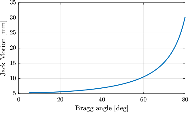
Figure 1: Jack motion as a function of Bragg angle
%% Required Jack stroke
ans = 1e3*(dz(end) - dz(1))
24.963
1.2. Kinematics (111 Crystal)
The reference frame is taken at the center of the 111 second crystal.
1.2.1. Interferometers - 111 Crystal
Three interferometers are pointed to the bottom surface of the 111 crystal.
The position of the measurement points are shown in Figure 2 as well as the origin where the motion of the crystal is computed.

Figure 2: Bottom view of the second crystal 111. Position of the measurement points.
The inverse kinematics consisting of deriving the interferometer measurements from the motion of the crystal (see Figure 3):
\begin{equation} \begin{bmatrix} x_1 \\ x_2 \\ x_3 \end{bmatrix} = \bm{J}_{s,111} \begin{bmatrix} d_z \\ r_y \\ r_x \end{bmatrix} \end{equation}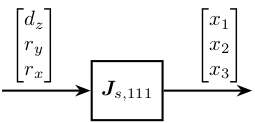
Figure 3: Inverse Kinematics - Interferometers
From the Figure 2, the inverse kinematics can be solved as follow (for small motion):
\begin{equation} \bm{J}_{s,111} = \begin{bmatrix} 1 & 0.07 & -0.015 \\ 1 & 0 & 0.015 \\ 1 & -0.07 & -0.015 \end{bmatrix} \end{equation}%% Sensor Jacobian matrix for 111 crystal J_s_111 = [1, 0.07, -0.015 1, 0, 0.015 1, -0.07, -0.015];
| 1.0 | 0.07 | -0.015 |
| 1.0 | 0.0 | 0.015 |
| 1.0 | -0.07 | -0.015 |
The forward kinematics is solved by inverting the Jacobian matrix (see Figure 4).
\begin{equation} \begin{bmatrix} d_z \\ r_y \\ r_x \end{bmatrix} = \bm{J}_{s,111}^{-1} \begin{bmatrix} x_1 \\ x_2 \\ x_3 \end{bmatrix} \end{equation}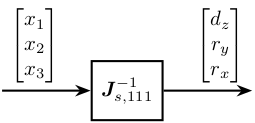
Figure 4: Forward Kinematics - Interferometers
| 0.25 | 0.5 | 0.25 |
| 7.14 | 0.0 | -7.14 |
| -16.67 | 33.33 | -16.67 |
1.2.2. Piezo - 111 Crystal
The location of the actuators with respect with the center of the 111 second crystal are shown in Figure 5.
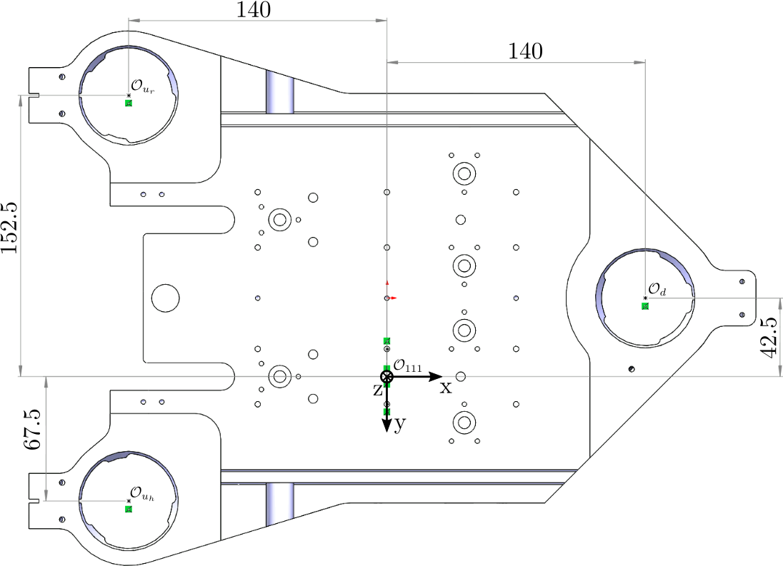
Figure 5: Location of actuators with respect to the center of the 111 second crystal (bottom view)
Inverse Kinematics consist of deriving the axial (z) motion of the 3 actuators from the motion of the crystal’s center.
\begin{equation} \begin{bmatrix} d_{u_r} \\ d_{u_h} \\ d_{d} \end{bmatrix} = \bm{J}_{a,111} \begin{bmatrix} d_z \\ r_y \\ r_x \end{bmatrix} \end{equation}
Figure 6: Inverse Kinematics - Actuators
Based on the geometry in Figure 5, we obtain:
\begin{equation} \bm{J}_{a,111} = \begin{bmatrix} 1 & 0.14 & -0.1525 \\ 1 & 0.14 & 0.0675 \\ 1 & -0.14 & -0.0425 \end{bmatrix} \end{equation}%% Actuator Jacobian - 111 crystal J_a_111 = [1, 0.14, -0.1525 1, 0.14, 0.0675 1, -0.14, -0.0425];
| 1.0 | 0.14 | -0.1525 |
| 1.0 | 0.14 | 0.0675 |
| 1.0 | -0.14 | -0.0425 |
The forward Kinematics is solved by inverting the Jacobian matrix:
\begin{equation} \begin{bmatrix} d_z \\ r_y \\ r_x \end{bmatrix} = \bm{J}_{a,111}^{-1} \begin{bmatrix} d_{u_r} \\ d_{u_h} \\ d_{d} \end{bmatrix} \end{equation}
Figure 7: Forward Kinematics - Actuators for 111 crystal
| 0.0568 | 0.4432 | 0.5 |
| 1.7857 | 1.7857 | -3.5714 |
| -4.5455 | 4.5455 | 0.0 |
1.3. Save Kinematics
save('mat/dcm_kinematics.mat', 'J_a_111', 'J_s_111')
2. Open Loop System Identification
2.1. Identification
Let’s considered the system \(\bm{G}(s)\) with:
- 3 inputs: force applied to the 3 fast jacks
- 3 outputs: measured displacement by the 3 interferometers pointing at the 111 second crystal
It is schematically shown in Figure 8.
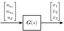
Figure 8: Dynamical system with inputs and outputs
The system is identified from the Simscape model.
%% Input/Output definition
clear io; io_i = 1;

%% Inputs
% Control Input {3x1} [N]
io(io_i) = linio([mdl, '/control_system'], 1, 'openinput');  io_i = io_i + 1;

%% Outputs
% Interferometers {3x1} [m]
io(io_i) = linio([mdl, '/DCM'], 1, 'openoutput'); io_i = io_i + 1;
%% Extraction of the dynamics
G = linearize(mdl, io);
size(G)
size(G)
State-space model with 3 outputs, 3 inputs, and 24 states.
2.2. Plant in the frame of the fastjacks
load('dcm_kinematics.mat');
Using the forward and inverse kinematics, we can computed the dynamics from piezo forces to axial motion of the 3 fastjacks (see Figure 9).
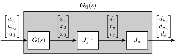
Figure 9: Use of Jacobian matrices to obtain the system in the frame of the fastjacks
%% Compute the system in the frame of the fastjacks
G_pz = J_a_111*inv(J_s_111)*G;
The DC gain of the new system shows that the system is well decoupled at low frequency.
dcgain(G_pz)
| 4.4407e-09 | 2.7656e-12 | 1.0132e-12 |
| 2.7656e-12 | 4.4407e-09 | 1.0132e-12 |
| 1.0109e-12 | 1.0109e-12 | 4.4424e-09 |
The bode plot of \(\bm{G}_{\text{fj}}(s)\) is shown in Figure 10.
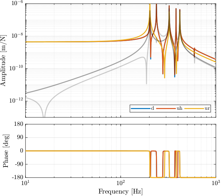
Figure 10: Bode plot of the diagonal and off-diagonal elements of the plant in the frame of the fast jacks
Computing the system in the frame of the fastjack gives good decoupling at low frequency (until the first resonance of the system).
2.3. Plant in the frame of the crystal
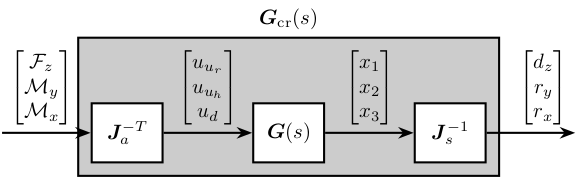
Figure 11: Use of Jacobian matrices to obtain the system in the frame of the crystal
G_mr = inv(J_s_111)*G*inv(J_a_111');
dcgain(G_mr)
| 1.9978e-09 | 3.9657e-09 | 7.7944e-09 |
| 3.9656e-09 | 8.4979e-08 | -1.5135e-17 |
| 7.7944e-09 | -3.9252e-17 | 1.834e-07 |
This results in a coupled system. The main reason is that, as we map forces to the center of the 111 crystal and not at the center of mass/stiffness of the moving part, vertical forces will induce rotation and torques will induce vertical motion.
3. Active Damping Plant (Strain gauges)
In this section, we wish to see whether if strain gauges fixed to the piezoelectric actuator can be used for active damping.
3.1. Identification
%% Input/Output definition
clear io; io_i = 1;

%% Inputs
% Control Input {3x1} [N]
io(io_i) = linio([mdl, '/control_system'], 1, 'openinput');  io_i = io_i + 1;

%% Outputs
% Strain Gauges {3x1} [m]
io(io_i) = linio([mdl, '/DCM'], 2, 'openoutput'); io_i = io_i + 1;
%% Extraction of the dynamics
G_sg = linearize(mdl, io);
dcgain(G_sg)
| 4.4443e-09 | 1.0339e-13 | 3.774e-14 |
| 1.0339e-13 | 4.4443e-09 | 3.774e-14 |
| 3.7792e-14 | 3.7792e-14 | 4.4444e-09 |
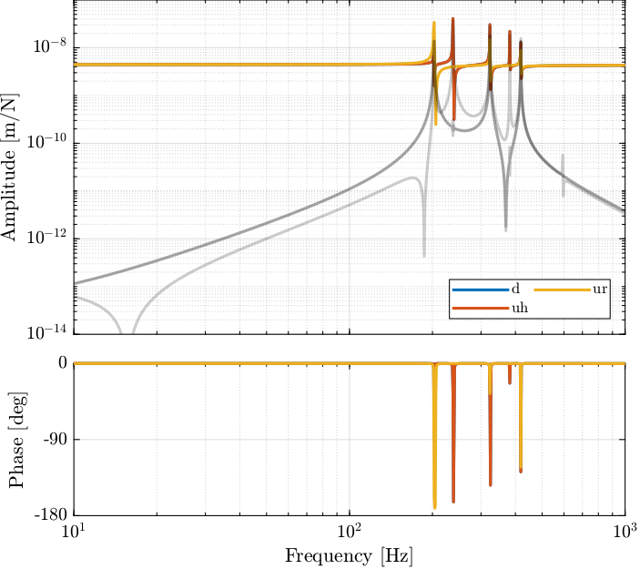
Figure 12: Bode Plot of the transfer functions from piezoelectric forces to strain gauges measuremed displacements
As the distance between the poles and zeros in Figure 15 is very small, little damping can be actively added using the strain gauges. This will be confirmed using a Root Locus plot.
3.2. Relative Active Damping
Krad_g1 = eye(3)*s/(s^2/(2*pi*500)^2 + 2*s/(2*pi*500) + 1);
As can be seen in Figure 13, very little damping can be added using relative damping strategy using strain gauges.

Figure 13: Root Locus for the relative damping control
Krad = -g*Krad_g1;
3.3. Damped Plant
The controller is implemented on Simscape, and the damped plant is identified.
%% Input/Output definition
clear io; io_i = 1;

%% Inputs
% Control Input {3x1} [N]
io(io_i) = linio([mdl, '/control_system'], 1, 'input');  io_i = io_i + 1;

%% Outputs
% Force Sensor {3x1} [m]
io(io_i) = linio([mdl, '/DCM'], 1, 'openoutput'); io_i = io_i + 1;
%% DCM Kinematics
load('dcm_kinematics.mat');
%% Identification of the Open Loop plant
controller.type = 0; % Open Loop
G_ol = J_a_111*inv(J_s_111)*linearize(mdl, io);
G_ol.InputName  = {'u_ur',  'u_uh',  'u_d'};
G_ol.OutputName = {'d_ur',  'd_uh',  'd_d'};
%% Identification of the damped plant with Relative Active Damping
controller.type = 2; % RAD
G_dp = J_a_111*inv(J_s_111)*linearize(mdl, io);
G_dp.InputName  = {'u_ur',  'u_uh',  'u_d'};
G_dp.OutputName = {'d_ur',  'd_uh',  'd_d'};
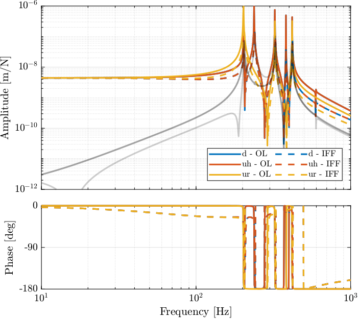
Figure 14: Bode plot of both the open-loop plant and the damped plant using relative active damping
4. Active Damping Plant (Force Sensors)
Force sensors are added above the piezoelectric actuators. They can consists of a simple piezoelectric ceramic stack. See for instance fleming10_integ_strain_force_feedb_high.
4.1. Identification
%% Input/Output definition
clear io; io_i = 1;

%% Inputs
% Control Input {3x1} [N]
io(io_i) = linio([mdl, '/control_system'], 1, 'openinput');  io_i = io_i + 1;

%% Outputs
% Force Sensor {3x1} [m]
io(io_i) = linio([mdl, '/DCM'], 3, 'openoutput'); io_i = io_i + 1;
%% Extraction of the dynamics
G_fs = linearize(mdl, io);
The Bode plot of the identified dynamics is shown in Figure 15. At high frequency, the diagonal terms are constants while the off-diagonal terms have some roll-off.
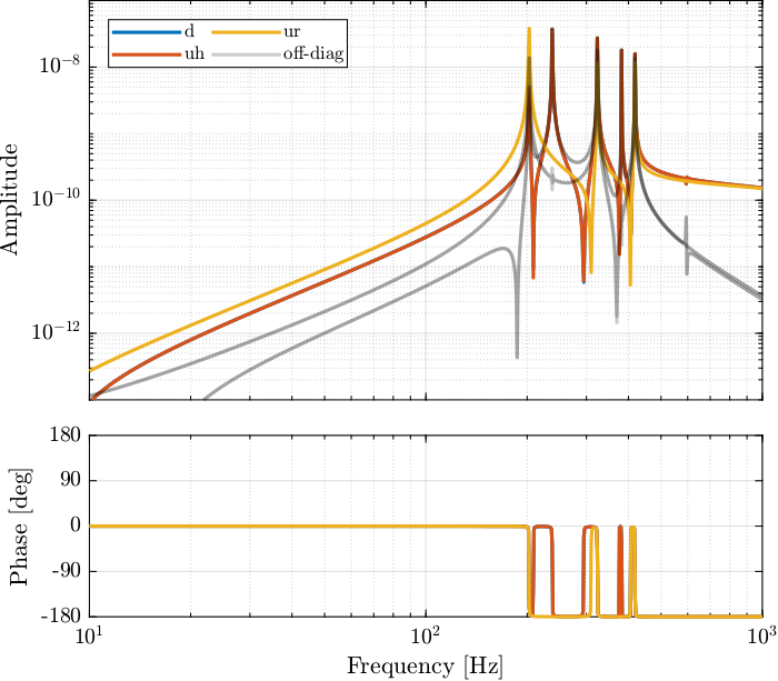
Figure 15: Bode plot of IFF Plant
4.2. Controller - Root Locus
We want to have integral action around the resonances of the system, but we do not want to integrate at low frequency. Therefore, we can use a low pass filter.
%% Integral Force Feedback Controller
Kiff_g1 = eye(3)*1/(1 + s/2/pi/20);
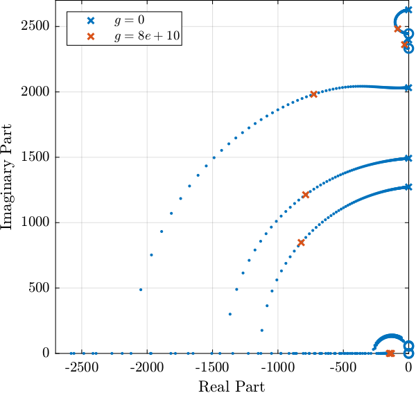
Figure 16: Root Locus plot for the IFF Control strategy
%% Integral Force Feedback Controller with optimal gain
Kiff = g*Kiff_g1;
%% Save the IFF controller
save('mat/Kiff.mat', 'Kiff');
4.3. Damped Plant
Both the Open Loop dynamics (see Figure 9) and the dynamics with IFF (see Figure 17) are identified.
We are here interested in the dynamics from \(\bm{u}^\prime = [u_{u_r}^\prime,\ u_{u_h}^\prime,\ u_d^\prime]\) (input of the damped plant) to \(\bm{d}_{\text{fj}} = [d_{u_r},\ d_{u_h},\ d_d]\) (motion of the crystal expressed in the frame of the fast-jacks). This is schematically represented in Figure 17.
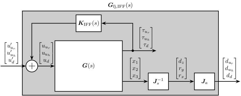
Figure 17: Use of Jacobian matrices to obtain the system in the frame of the fastjacks
The dynamics from \(\bm{u}\) to \(\bm{d}_{\text{fj}}\) (open-loop dynamics) and from \(\bm{u}^\prime\) to \(\bm{d}_{\text{fs}}\) are compared in Figure 18. It is clear that the Integral Force Feedback control strategy is very effective in damping the resonances of the plant.
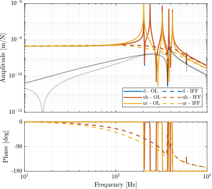
Figure 18: Bode plot of both the open-loop plant and the damped plant using IFF
The Integral Force Feedback control strategy is very effective in damping the modes present in the plant.
5. HAC-LAC (IFF) architecture
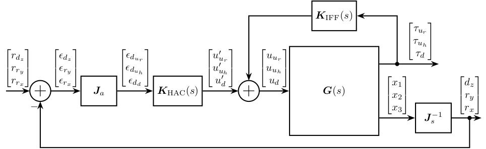
5.1. System Identification
Let’s identify the damped plant.
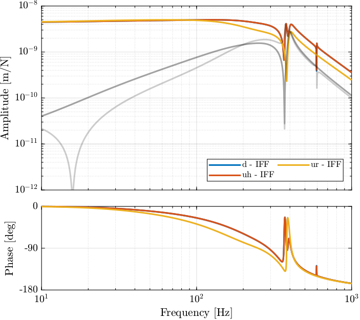
Figure 20: Bode Plot of the plant for the High Authority Controller (transfer function from \(\bm{u}^\prime\) to \(\bm{\epsilon}_d\))
5.2. High Authority Controller
Let’s design a controller with a bandwidth of 100Hz. As the plant is well decoupled and well approximated by a constant at low frequency, the high authority controller can easily be designed with SISO loop shaping.
%% Controller design
wc = 2*pi*100; % Wanted crossover frequency [rad/s]
a = 2; % Lead parameter

Khac = diag(1./diag(abs(evalfr(G_dp, 1j*wc)))) * ... % Diagonal controller
        wc/s * ... % Integrator
        1/(sqrt(a))*(1 + s/(wc/sqrt(a)))/(1 + s/(wc*sqrt(a))) * ... % Lead
        1/(s^2/(4*wc)^2 + 2*s/(4*wc) + 1); % Low pass filter
%% Save the HAC controller
save('mat/Khac_iff.mat', 'Khac');
%% Loop Gain
L_hac_lac = G_dp * Khac;
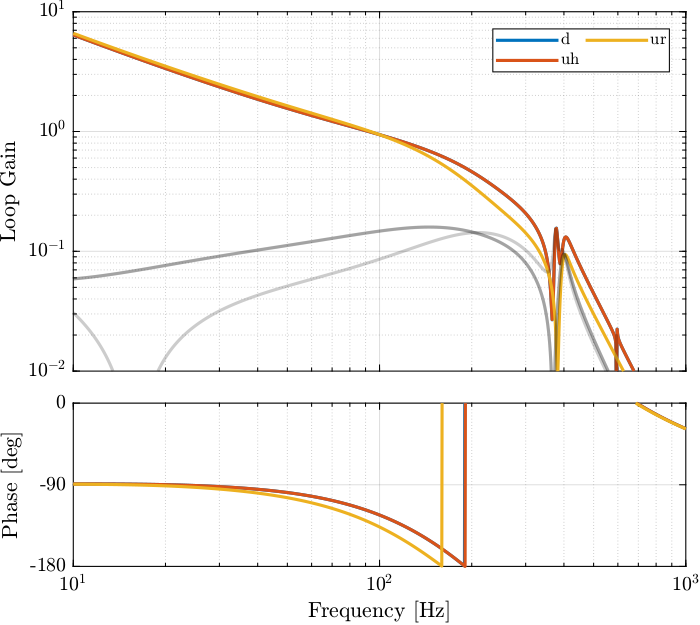
Figure 21: Bode Plot of the Loop gain for the High Authority Controller
As shown in the Root Locus plot in Figure 22, the closed loop system should be stable.
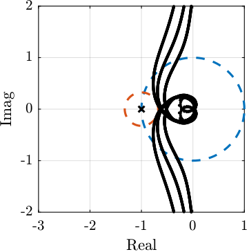
Figure 22: Root Locus for the High Authority Controller
5.3. Performances
In order to estimate the performances of the HAC-IFF control strategy, the transfer function from motion errors of the stepper motors to the motion error of the crystal is identified both in open loop and with the HAC-IFF strategy.
It is first verified that the closed-loop system is stable:
isstable(T_hl)
1
And both transmissibilities are compared in Figure 23.
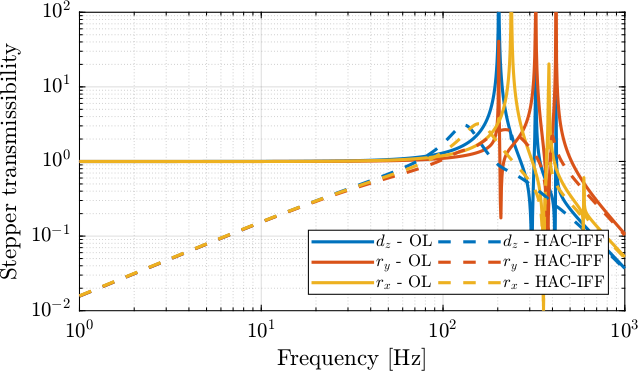
Figure 23: Comparison of the transmissibility of errors from vibrations of the stepper motor between the open-loop case and the hac-iff case.
The HAC-IFF control strategy can effectively reduce the transmissibility of the motion errors of the stepper motors. This reduction is effective inside the bandwidth of the controller.