Encoder Renishaw Vionic - Test Bench
Table of Contents
This report is also available as a pdf.
You can find below the document of:
We would like to characterize the encoder measurement system.
In particular, we would like to measure:
- Power Spectral Density of the measurement noise
- Bandwidth of the sensor
- Linearity of the sensor
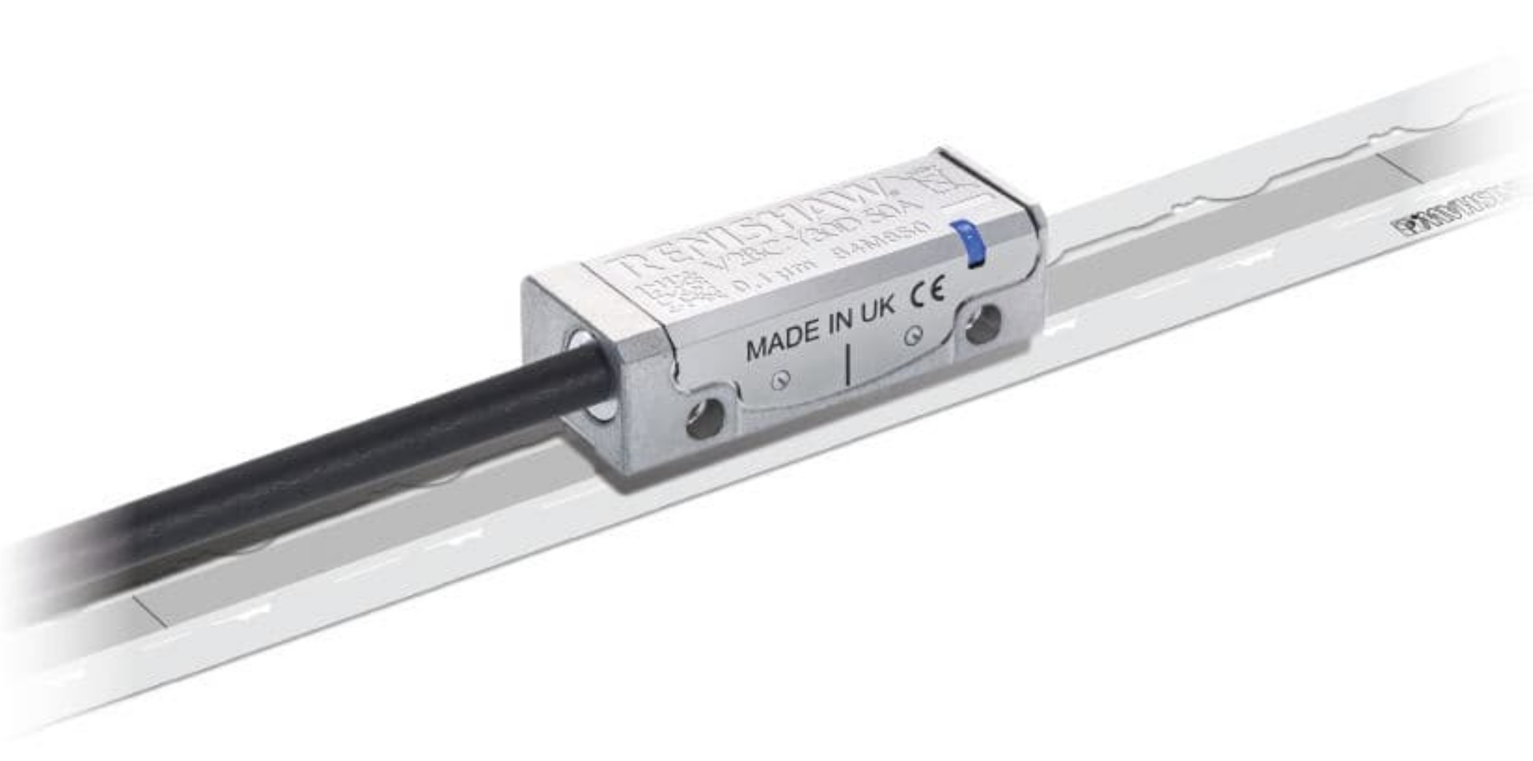
Figure 1: Picture of the Vionic Encoder
- 1: 2YA275
- 2: 2YA274
- 3: 2YA273
- 4: 2YA270
- 5: 2YA272
- 6: 2YA271
- 7: 2YJ313
1 Encoder Model
The Encoder is characterized by its dynamics \(G_m(s)\) from the “true” displacement \(y\) to measured displacement \(y_m\). Ideally, this dynamics is constant over a wide frequency band with very small phase drop.
It is also characterized by its measurement noise \(n\) that can be described by its Power Spectral Density (PSD).
The model of the encoder is shown in Figure 2.
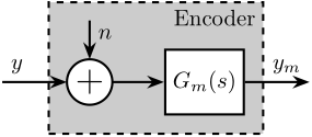
Figure 2: Model of the Encoder
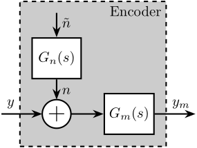
We can also use a transfer function \(G_n(s)\) to shape a noise \(\tilde{n}\) with unity ASD as shown in Figure 4.
| Characteristics | Manual | Specifications |
|---|---|---|
| Range | Ruler length | > 200 [um] |
| Resolution | 2.5 [nm] | < 50 [nm rms] |
| Sub-Divisional Error | \(< \pm 15\,nm\) | |
| Bandwidth | To be checked | > 5 [kHz] |
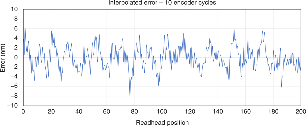
Figure 4: Expected interpolation errors for the Vionic Encoder
2 Noise Measurement
2.1 Test Bench
To measure the noise \(n\) of the encoder, one can rigidly fix the head and the ruler together such that no motion should be measured. Then, the measured signal \(y_m\) corresponds to the noise \(n\).
2.2 Results
First we load the data.
%% Load Data
enc1 = load('noise_meas_100s_20kHz_1.mat', 't', 'x');
enc2 = load('noise_meas_100s_20kHz_2.mat', 't', 'x');
enc3 = load('noise_meas_100s_20kHz_3.mat', 't', 'x');
enc4 = load('noise_meas_100s_20kHz_4.mat', 't', 'x');
enc6 = load('noise_meas_100s_20kHz_6.mat', 't', 'x');
enc7 = load('noise_meas_100s_20kHz_7.mat', 't', 'x');
The raw measured data as well as the low pass filtered data (using a first order low pass filter with a cut-off at 10Hz) are shown in Figure 5.
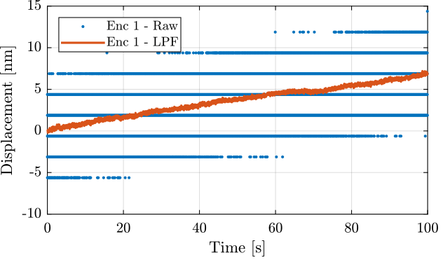
Figure 5: Time domain measurement (raw data and low pass filtered data with first order 10Hz LPF)
The time domain data for all the encoders are compared in Figure 6.
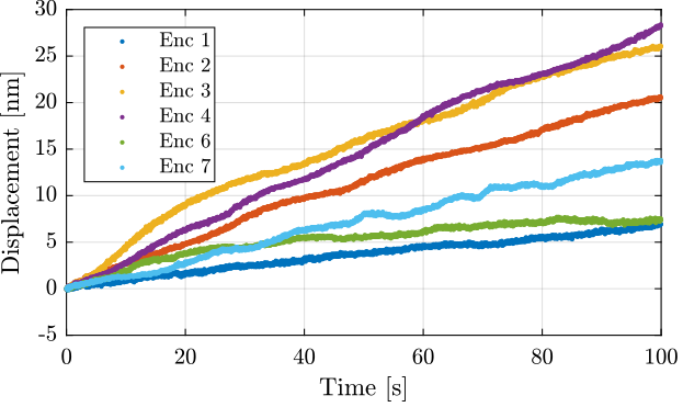
Figure 6: Comparison of the time domain measurement
The amplitude spectral density is computed and shown in Figure 7.
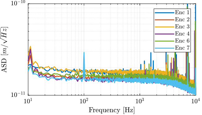
Figure 7: Amplitude Spectral Density of the measured signal
Let’s create a transfer function that approximate the measured noise of the encoder.
Gn_e = 1.8e-11/(1 + s/2/pi/1e4);
The amplitude of the transfer function and the measured ASD are shown in Figure 8.
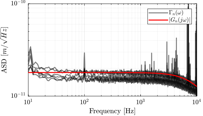
Figure 8: Measured ASD of the noise and modelled one
3 Linearity Measurement
3.1 Test Bench
In order to measure the linearity, we have to compare the measured displacement with a reference sensor with a known linearity. An interferometer or capacitive sensor should work fine. An actuator should also be there so impose a displacement.
One idea is to use the test-bench shown in Figure 9.
The APA300ML is used to excite the mass in a broad bandwidth. The motion is measured at the same time by the Vionic Encoder and by an interferometer (most likely an Attocube).
As the interferometer has a very large bandwidth, we should be able to estimate the bandwidth of the encoder if it is less than the Nyquist frequency that can be around 10kHz.
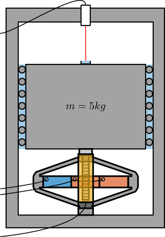
Figure 9: Schematic of the test bench