Nano-Hexapod - Test Bench

1. Encoders fixed to the Struts

This report is also available as a pdf.

Here are the documentation of the equipment used for this test bench:

Voltage Amplifier: PiezoDrive PD200
Amplified Piezoelectric Actuator: Cedrat APA300ML
DAC/ADC: Speedgoat IO313
Encoder: Renishaw Vionic and used Ruler
Interferometers: Attocube

Figure 1: Nano-Hexapod

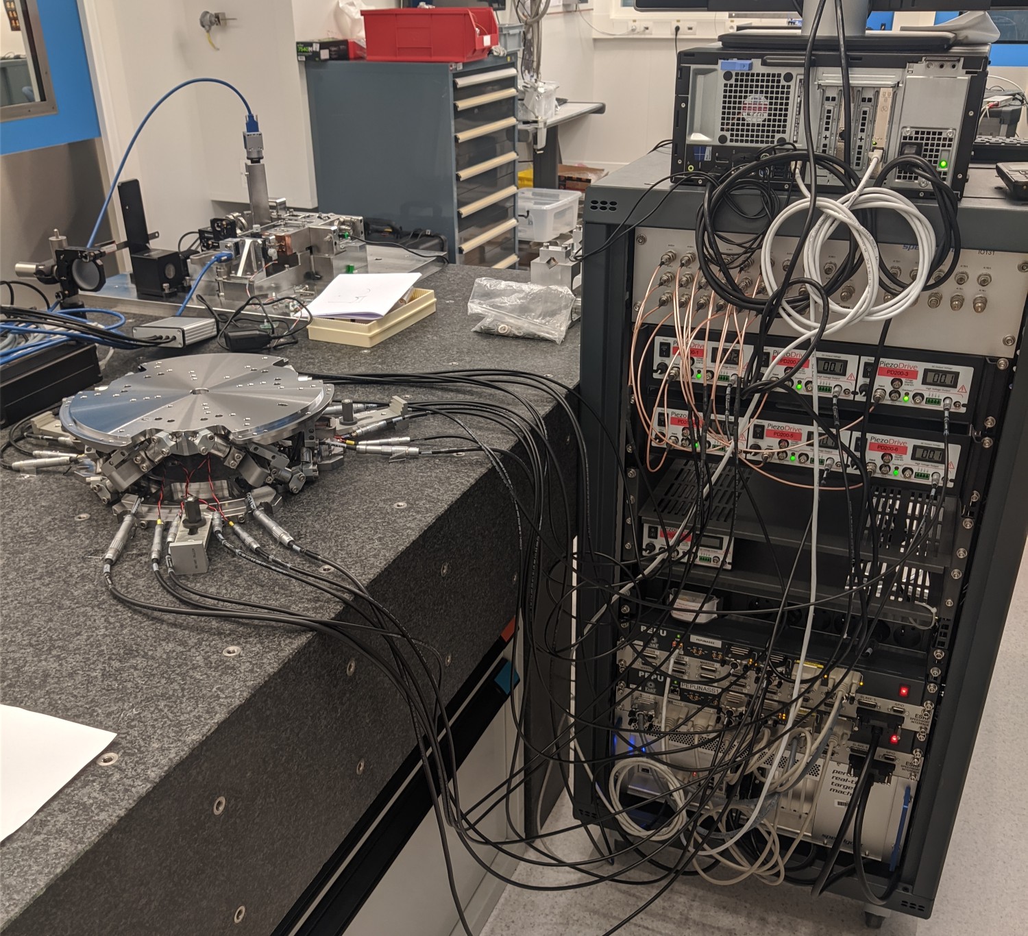
Figure 2: Nano-Hexapod and the control electronics

1 Encoders fixed to the Struts

1.1 Introduction

In this section, the encoders are fixed to the struts.

1.2 Load Data

meas_data_lf = {};

for i = 1:6
    meas_data_lf(i) = {load(sprintf('mat/frf_data_exc_strut_%i_noise_lf.mat', i), 't', 'Va', 'Vs', 'de')};
    meas_data_hf(i) = {load(sprintf('mat/frf_data_exc_strut_%i_noise_hf.mat', i), 't', 'Va', 'Vs', 'de')};
end

1.3 Spectral Analysis - Setup

% Sampling Time [s]
Ts = (meas_data_lf{1}.t(end) - (meas_data_lf{1}.t(1)))/(length(meas_data_lf{1}.t)-1);

% Sampling Frequency [Hz]
Fs = 1/Ts;

% Hannning Windows
win = hanning(ceil(1*Fs));

And we get the frequency vector.

[~, f] = tfestimate(meas_data_lf{1}.Va, meas_data_lf{1}.de, win, [], [], 1/Ts);

i_lf = f < 250; % Points for low frequency excitation
i_hf = f > 250; % Points for high frequency excitation

1.4 DVF Plant

First, let’s compute the coherence from the excitation voltage and the displacement as measured by the encoders (Figure 3).

%% Coherence
coh_dvf_lf = zeros(length(f), 6, 6);
coh_dvf_hf = zeros(length(f), 6, 6);

for i = 1:6
    coh_dvf_lf(:, :, i) = mscohere(meas_data_lf{i}.Va, meas_data_lf{i}.de, win, [], [], 1/Ts);
    coh_dvf_hf(:, :, i) = mscohere(meas_data_hf{i}.Va, meas_data_hf{i}.de, win, [], [], 1/Ts);
end

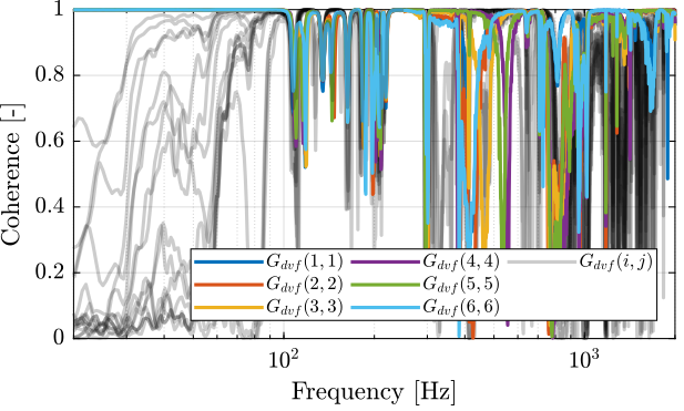
Figure 3: Obtained coherence for the DVF plant

Then the 6x6 transfer function matrix is estimated (Figure 4).

%% DVF Plant
G_dvf_lf = zeros(length(f), 6, 6);
G_dvf_hf = zeros(length(f), 6, 6);

for i = 1:6
    G_dvf_lf(:, :, i) = tfestimate(meas_data_lf{i}.Va, meas_data_lf{i}.de, win, [], [], 1/Ts);
    G_dvf_hf(:, :, i) = tfestimate(meas_data_hf{i}.Va, meas_data_hf{i}.de, win, [], [], 1/Ts);
end

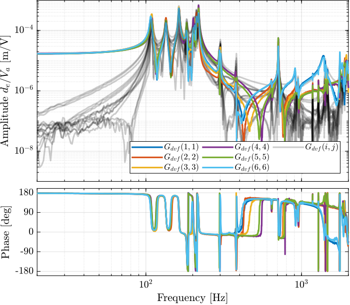
Figure 4: Measured FRF for the DVF plant

1.5 IFF Plant

First, let’s compute the coherence from the excitation voltage and the displacement as measured by the encoders (Figure 5).

%% Coherence
coh_iff_lf = zeros(length(f), 6, 6);
coh_iff_hf = zeros(length(f), 6, 6);

for i = 1:6
    coh_iff_lf(:, :, i) = mscohere(meas_data_lf{i}.Va, meas_data_lf{i}.Vs, win, [], [], 1/Ts);
    coh_iff_hf(:, :, i) = mscohere(meas_data_hf{i}.Va, meas_data_hf{i}.Vs, win, [], [], 1/Ts);
end

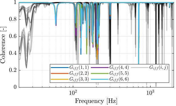
Figure 5: Obtained coherence for the IFF plant

Then the 6x6 transfer function matrix is estimated (Figure 6).

%% IFF Plant
G_iff_lf = zeros(length(f), 6, 6);
G_iff_hf = zeros(length(f), 6, 6);

for i = 1:6
    G_iff_lf(:, :, i) = tfestimate(meas_data_lf{i}.Va, meas_data_lf{i}.Vs, win, [], [], 1/Ts);
    G_iff_hf(:, :, i) = tfestimate(meas_data_hf{i}.Va, meas_data_hf{i}.Vs, win, [], [], 1/Ts);
end

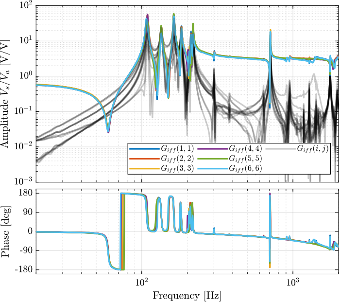
Figure 6: Measured FRF for the IFF plant

1.6 Jacobian

The Jacobian is used to transform the excitation force in the cartesian frame as well as the displacements.

Consider the plant shown in Figure 7 with:

\(\tau\) the 6 input voltages (going to the PD200 amplifier and then to the APA)
\(d\mathcal{L}\) the relative motion sensor outputs (encoders)
\(\bm{\tau}_m\) the generated voltage of the force sensor stacks
\(J_a\) and \(J_s\) the Jacobians for the actuators and sensors

Figure 7: Plant in the cartesian Frame

First, we load the Jacobian matrix (same for the actuators and sensors).

load('jacobian.mat', 'J');

1.6.1 DVF Plant

The transfer function from \(\bm{\mathcal{F}}\) to \(d\bm{\mathcal{X}}\) is computed and shown in Figure 8.

G_dvf_J_lf = permute(pagemtimes(inv(J), pagemtimes(permute(G_dvf_lf, [2 3 1]), inv(J'))), [3 1 2]);
G_dvf_J_hf = permute(pagemtimes(inv(J), pagemtimes(permute(G_dvf_hf, [2 3 1]), inv(J'))), [3 1 2]);

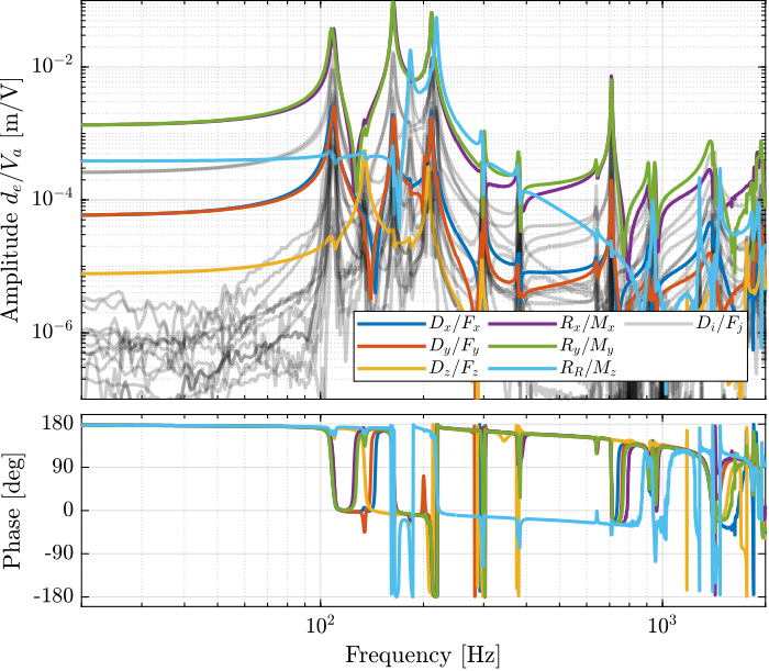
Figure 8: Measured FRF for the DVF plant in the cartesian frame

1.6.2 IFF Plant

The transfer function from \(\bm{\mathcal{F}}\) to \(\bm{\mathcal{F}}_m\) is computed and shown in Figure 9.

G_iff_J_lf = permute(pagemtimes(inv(J), pagemtimes(permute(G_iff_lf, [2 3 1]), inv(J'))), [3 1 2]);
G_iff_J_hf = permute(pagemtimes(inv(J), pagemtimes(permute(G_iff_hf, [2 3 1]), inv(J'))), [3 1 2]);

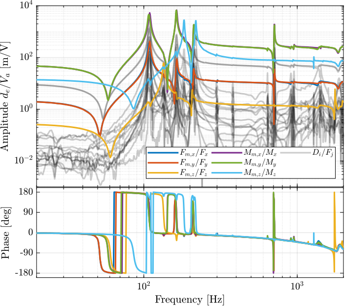
Figure 9: Measured FRF for the IFF plant in the cartesian frame