Nano-Hexapod - Test Bench

1. Encoders fixed to the Struts
2. Encoders fixed to the plates

This report is also available as a pdf.

In this document, the dynamics of the nano-hexapod shown in Figure 1 is identified.

Here are the documentation of the equipment used for this test bench:

Voltage Amplifier: PiezoDrive PD200
Amplified Piezoelectric Actuator: Cedrat APA300ML
DAC/ADC: Speedgoat IO313
Encoder: Renishaw Vionic and used Ruler
Interferometers: Attocube

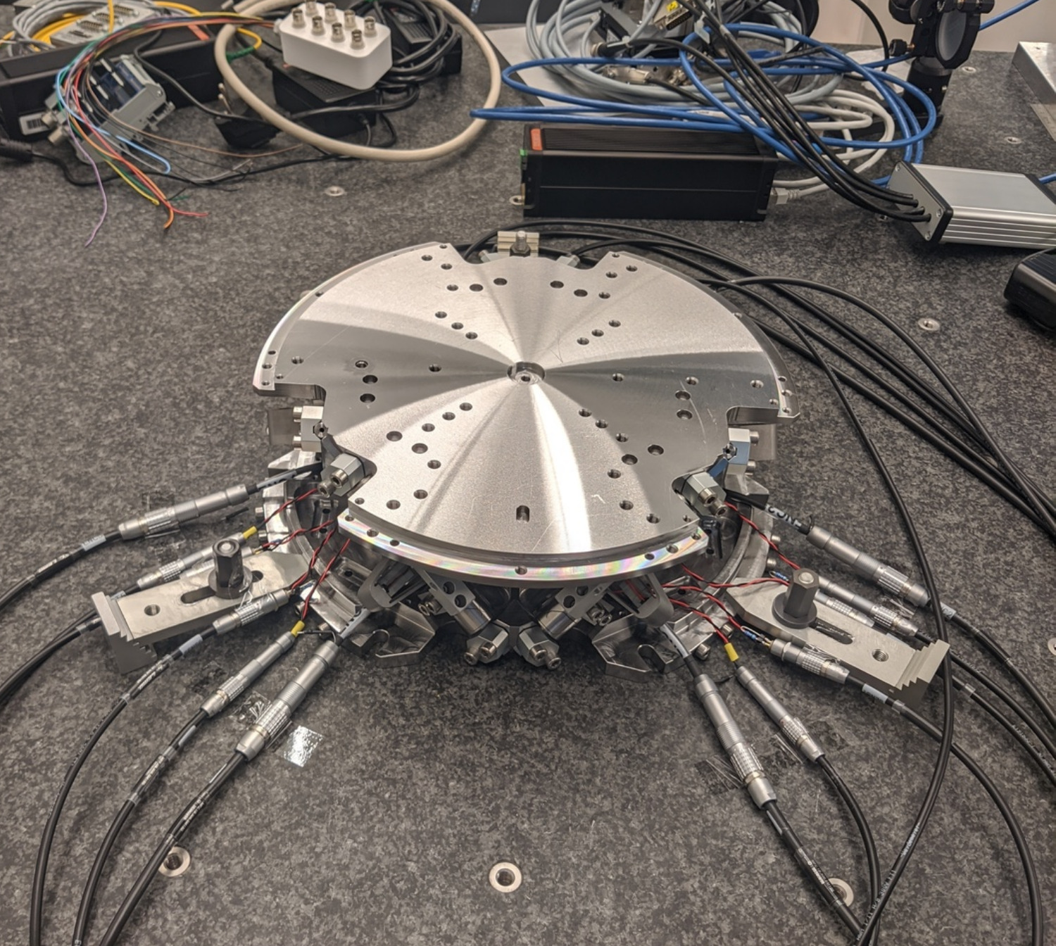
Figure 1: Nano-Hexapod

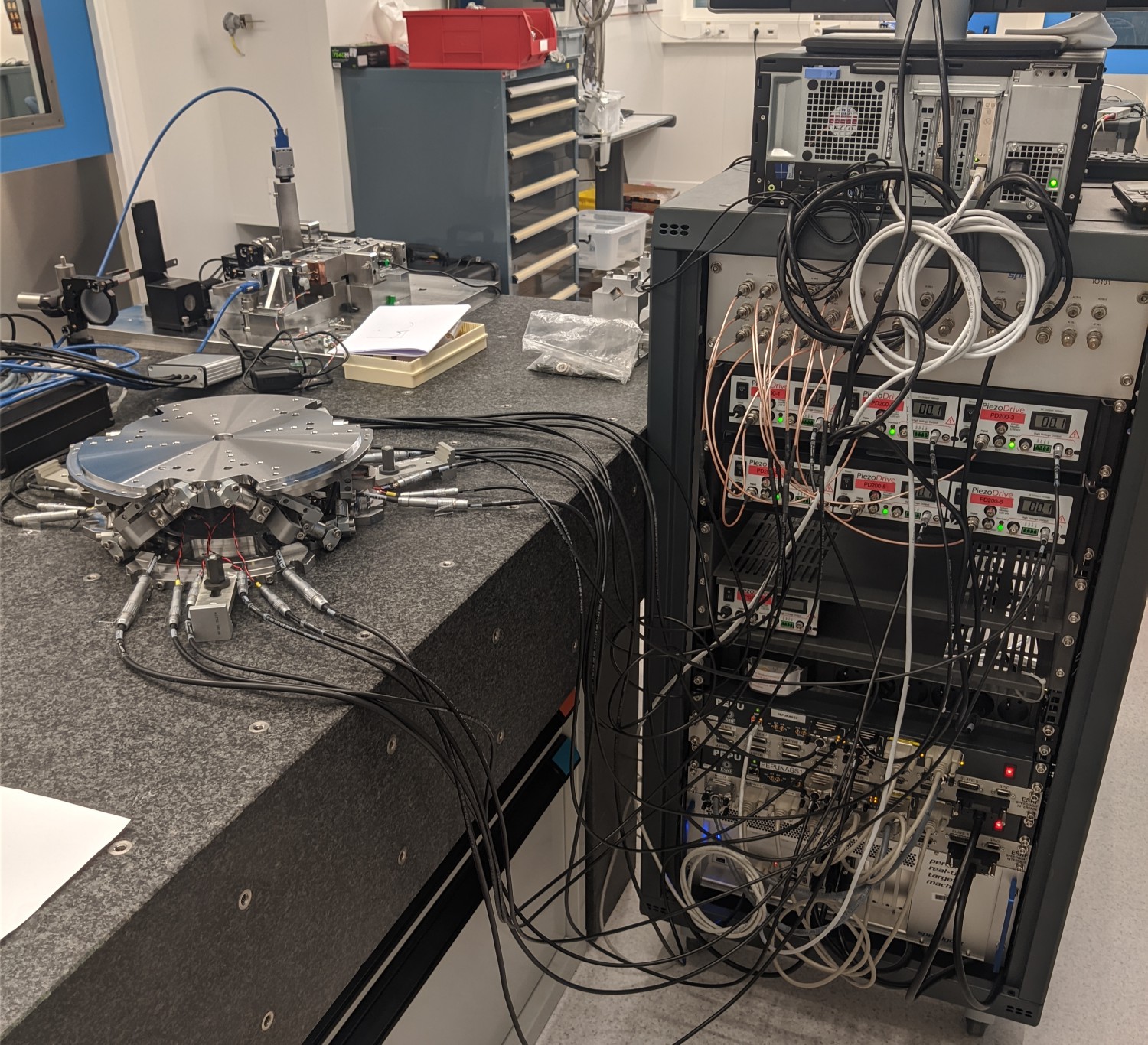
Figure 2: Nano-Hexapod and the control electronics

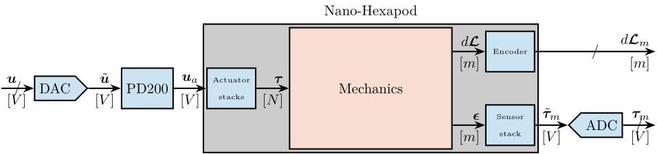
Figure 3: Block diagram of the system with named signals

Table 1: List of signals
	Unit	Matlab	Vector	Elements
Control Input (wanted DAC voltage)	`[V]`	`u`	\(\bm{u}\)	\(u_i\)
DAC Output Voltage	`[V]`	`u`	\(\tilde{\bm{u}}\)	\(\tilde{u}_i\)
PD200 Output Voltage	`[V]`	`ua`	\(\bm{u}_a\)	\(u_{a,i}\)
Actuator applied force	`[N]`	`tau`	\(\bm{\tau}\)	\(\tau_i\)
Strut motion	`[m]`	`dL`	\(d\bm{\mathcal{L}}\)	\(d\mathcal{L}_i\)
Encoder measured displacement	`[m]`	`dLm`	\(d\bm{\mathcal{L}}_m\)	\(d\mathcal{L}_{m,i}\)
Force Sensor strain	`[m]`	`epsilon`	\(\bm{\epsilon}\)	\(\epsilon_i\)
Force Sensor Generated Voltage	`[V]`	`taum`	\(\tilde{\bm{\tau}}_m\)	\(\tilde{\tau}_{m,i}\)
Measured Generated Voltage	`[V]`	`taum`	\(\bm{\tau}_m\)	\(\tau_{m,i}\)
Motion of the top platform	`[m,rad]`	`dX`	\(d\bm{\mathcal{X}}\)	\(d\mathcal{X}_i\)
Metrology measured displacement	`[m,rad]`	`dXm`	\(d\bm{\mathcal{X}}_m\)	\(d\mathcal{X}_{m,i}\)

1 Encoders fixed to the Struts

1.1 Introduction

In this section, the encoders are fixed to the struts.

1.2 Identification of the dynamics

1.2.1 Load Data

%% Load Identification Data
meas_data_lf = {};

for i = 1:6
    meas_data_lf(i) = {load(sprintf('mat/frf_data_exc_strut_%i_noise_lf.mat', i), 't', 'Va', 'Vs', 'de')};
    meas_data_hf(i) = {load(sprintf('mat/frf_data_exc_strut_%i_noise_hf.mat', i), 't', 'Va', 'Vs', 'de')};
end

1.2.2 Spectral Analysis - Setup

%% Setup useful variables
% Sampling Time [s]
Ts = (meas_data_lf{1}.t(end) - (meas_data_lf{1}.t(1)))/(length(meas_data_lf{1}.t)-1);

% Sampling Frequency [Hz]
Fs = 1/Ts;

% Hannning Windows
win = hanning(ceil(1*Fs));

% And we get the frequency vector
[~, f] = tfestimate(meas_data_lf{1}.Va, meas_data_lf{1}.de, win, [], [], 1/Ts);

i_lf = f < 250; % Points for low frequency excitation
i_hf = f > 250; % Points for high frequency excitation

1.2.3 DVF Plant

First, let’s compute the coherence from the excitation voltage and the displacement as measured by the encoders (Figure 4).

%% Coherence
coh_dvf_lf = zeros(length(f), 6, 6);
coh_dvf_hf = zeros(length(f), 6, 6);

for i = 1:6
    coh_dvf_lf(:, :, i) = mscohere(meas_data_lf{i}.Va, meas_data_lf{i}.de, win, [], [], 1/Ts);
    coh_dvf_hf(:, :, i) = mscohere(meas_data_hf{i}.Va, meas_data_hf{i}.de, win, [], [], 1/Ts);
end

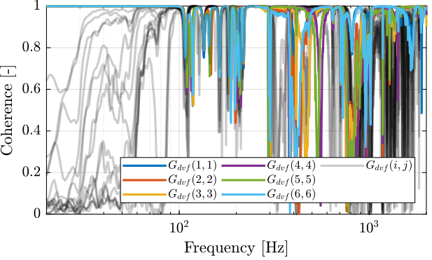
Figure 4: Obtained coherence for the DVF plant

Then the 6x6 transfer function matrix is estimated (Figure 5).

%% DVF Plant (transfer function from u to dLm)
G_dvf_lf = zeros(length(f), 6, 6);
G_dvf_hf = zeros(length(f), 6, 6);

for i = 1:6
    G_dvf_lf(:, :, i) = tfestimate(meas_data_lf{i}.Va, meas_data_lf{i}.de, win, [], [], 1/Ts);
    G_dvf_hf(:, :, i) = tfestimate(meas_data_hf{i}.Va, meas_data_hf{i}.de, win, [], [], 1/Ts);
end

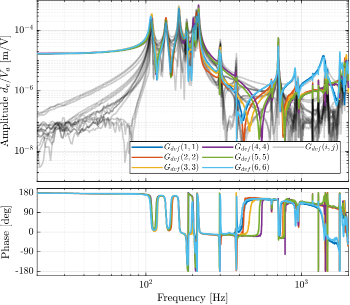
Figure 5: Measured FRF for the DVF plant

1.2.4 IFF Plant

First, let’s compute the coherence from the excitation voltage and the displacement as measured by the encoders (Figure 6).

%% Coherence for the IFF plant
coh_iff_lf = zeros(length(f), 6, 6);
coh_iff_hf = zeros(length(f), 6, 6);

for i = 1:6
    coh_iff_lf(:, :, i) = mscohere(meas_data_lf{i}.Va, meas_data_lf{i}.Vs, win, [], [], 1/Ts);
    coh_iff_hf(:, :, i) = mscohere(meas_data_hf{i}.Va, meas_data_hf{i}.Vs, win, [], [], 1/Ts);
end

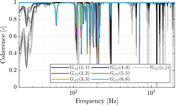
Figure 6: Obtained coherence for the IFF plant

Then the 6x6 transfer function matrix is estimated (Figure 7).

%% IFF Plant
G_iff_lf = zeros(length(f), 6, 6);
G_iff_hf = zeros(length(f), 6, 6);

for i = 1:6
    G_iff_lf(:, :, i) = tfestimate(meas_data_lf{i}.Va, meas_data_lf{i}.Vs, win, [], [], 1/Ts);
    G_iff_hf(:, :, i) = tfestimate(meas_data_hf{i}.Va, meas_data_hf{i}.Vs, win, [], [], 1/Ts);
end

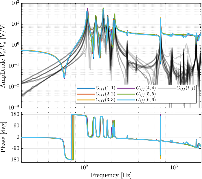
Figure 7: Measured FRF for the IFF plant

1.3 Comparison with the Simscape Model

In this section, the measured dynamics is compared with the dynamics estimated from the Simscape model.

1.3.1 Dynamics from Actuator to Force Sensors

%% Initialize Nano-Hexapod
n_hexapod = initializeNanoHexapodFinal('flex_bot_type', '4dof', ...
                                       'flex_top_type', '4dof', ...
                                       'motion_sensor_type', 'struts', ...
                                       'actuator_type', '2dof');

%% Identify the IFF Plant (transfer function from u to taum)
clear io; io_i = 1;
io(io_i) = linio([mdl, '/F'],  1, 'openinput');   io_i = io_i + 1; % Actuator Inputs
io(io_i) = linio([mdl, '/Fm'],  1, 'openoutput'); io_i = io_i + 1; % Force Sensors

Giff = exp(-s*Ts)*linearize(mdl, io, 0.0, options);

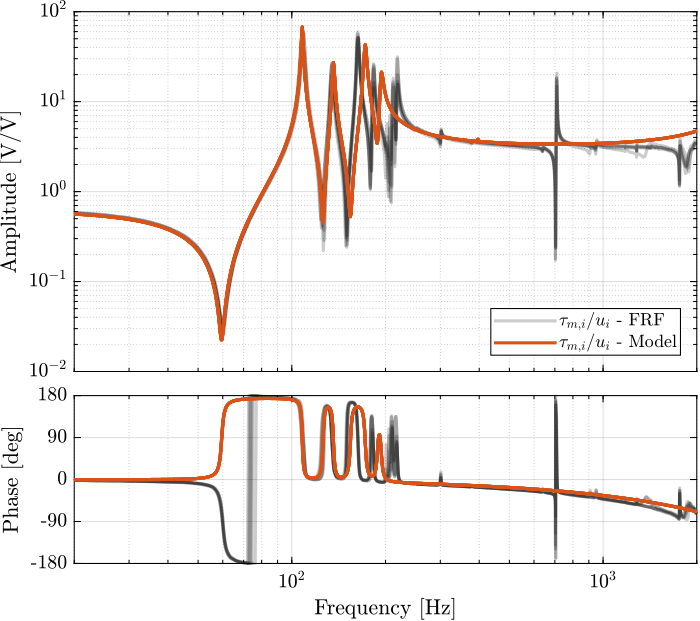
Figure 8: Diagonal elements of the IFF Plant

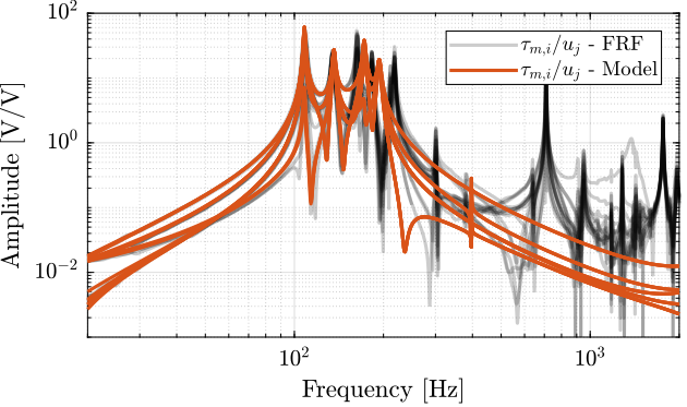
Figure 9: Off diagonal elements of the IFF Plant

1.3.2 Dynamics from Actuator to Encoder

%% Initialization of the Nano-Hexapod
n_hexapod = initializeNanoHexapodFinal('flex_bot_type', '4dof', ...
                                       'flex_top_type', '4dof', ...
                                       'motion_sensor_type', 'struts', ...
                                       'actuator_type', '2dof');

%% Identify the DVF Plant (transfer function from u to dLm)
clear io; io_i = 1;
io(io_i) = linio([mdl, '/F'],  1, 'openinput');  io_i = io_i + 1; % Actuator Inputs
io(io_i) = linio([mdl, '/D'],  1, 'openoutput'); io_i = io_i + 1; % Encoders

Gdvf = exp(-s*Ts)*linearize(mdl, io, 0.0, options);

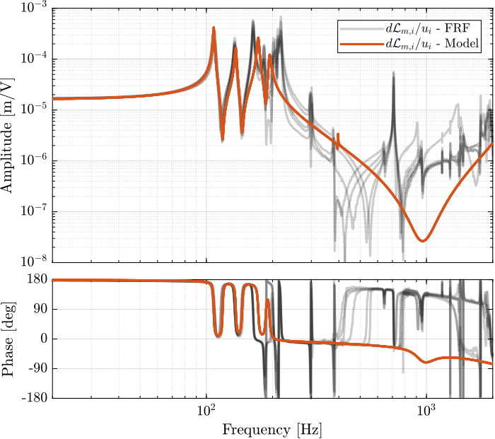
Figure 10: Diagonal elements of the DVF Plant

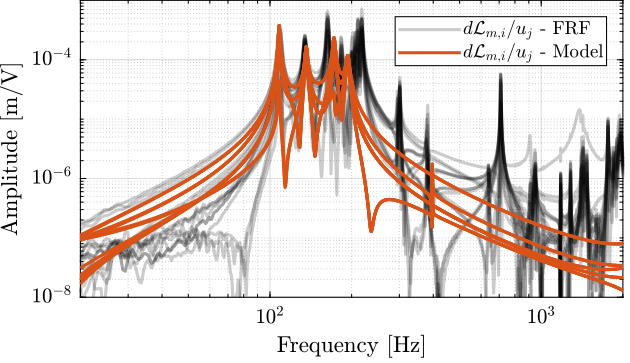
Figure 11: Off diagonal elements of the DVF Plant

1.4 Integral Force Feedback

1.4.1 Root Locus and Decentralized Loop gain

%% IFF Controller
Kiff_g1 = (1/(s + 2*pi*40))*... % Low pass filter (provides integral action above 40Hz)
          (s/(s + 2*pi*30))*... % High pass filter to limit low frequency gain
          (1/(1 + s/2/pi/500))*... % Low pass filter to be more robust to high frequency resonances
          eye(6); % Diagonal 6x6 controller

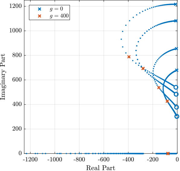
Figure 12: Root Locus for the IFF control strategy

Then the “optimal” IFF controller is:

%% IFF controller with Optimal gain
Kiff = g*Kiff_g1;

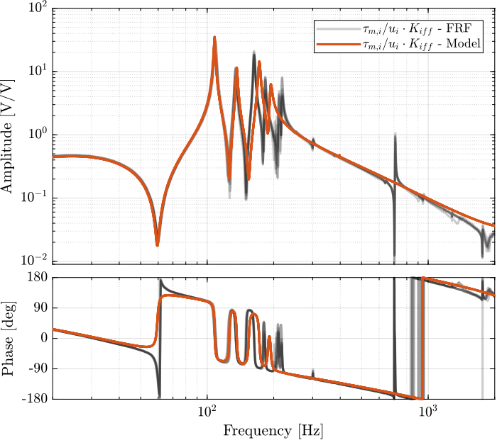
Figure 13: Bode plot of the “decentralized loop gain” \(G_\text{iff}(i,i) \times K_\text{iff}(i,i)\)

1.4.2 Multiple Gains - Simulation

%% Tested IFF gains
iff_gains = [4, 10, 20, 40, 100, 200, 400];

%% Initialize the Simscape model in closed loop
n_hexapod = initializeNanoHexapodFinal('flex_bot_type', '4dof', ...
                                       'flex_top_type', '4dof', ...
                                       'motion_sensor_type', 'struts', ...
                                       'actuator_type', '2dof', ...
                                       'controller_type', 'iff');

%% Identify the (damped) transfer function from u to dLm for different values of the IFF gain
Gd_iff = {zeros(1, length(iff_gains))};

clear io; io_i = 1;
io(io_i) = linio([mdl, '/F'],  1, 'openinput');  io_i = io_i + 1; % Actuator Inputs
io(io_i) = linio([mdl, '/D'],  1, 'openoutput'); io_i = io_i + 1; % Strut Displacement (encoder)

for i = 1:length(iff_gains)
    Kiff = iff_gains(i)*Kiff_g1*eye(6); % IFF Controller
    Gd_iff(i) = {exp(-s*Ts)*linearize(mdl, io, 0.0, options)};

    isstable(Gd_iff{i})
end

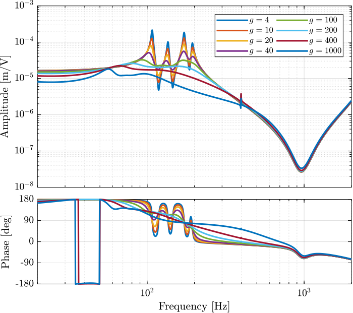
Figure 14: Effect of the IFF gain \(g\) on the transfer function from \(\bm{\tau}\) to \(d\bm{\mathcal{L}}_m\)

1.4.3 Experimental Results - Gains

Let’s look at the damping introduced by IFF as a function of the IFF gain and compare that with the results obtained using the Simscape model.

1.4.3.1 Load Data

%% Load Identification Data
meas_iff_gains = {};

for i = 1:length(iff_gains)
    meas_iff_gains(i) = {load(sprintf('mat/iff_strut_1_noise_g_%i.mat', iff_gains(i)), 't', 'Vexc', 'Vs', 'de', 'u')};
end

1.4.3.2 Spectral Analysis - Setup

%% Setup useful variables
% Sampling Time [s]
Ts = (meas_iff_gains{1}.t(end) - (meas_iff_gains{1}.t(1)))/(length(meas_iff_gains{1}.t)-1);

% Sampling Frequency [Hz]
Fs = 1/Ts;

% Hannning Windows
win = hanning(ceil(1*Fs));

% And we get the frequency vector
[~, f] = tfestimate(meas_iff_gains{1}.Vexc, meas_iff_gains{1}.de, win, [], [], 1/Ts);

1.4.3.3 DVF Plant

%% DVF Plant (transfer function from u to dLm)
G_iff_gains = {};

for i = 1:length(iff_gains)
    G_iff_gains{i} = tfestimate(meas_iff_gains{i}.Vexc, meas_iff_gains{i}.de(:,1), win, [], [], 1/Ts);
end

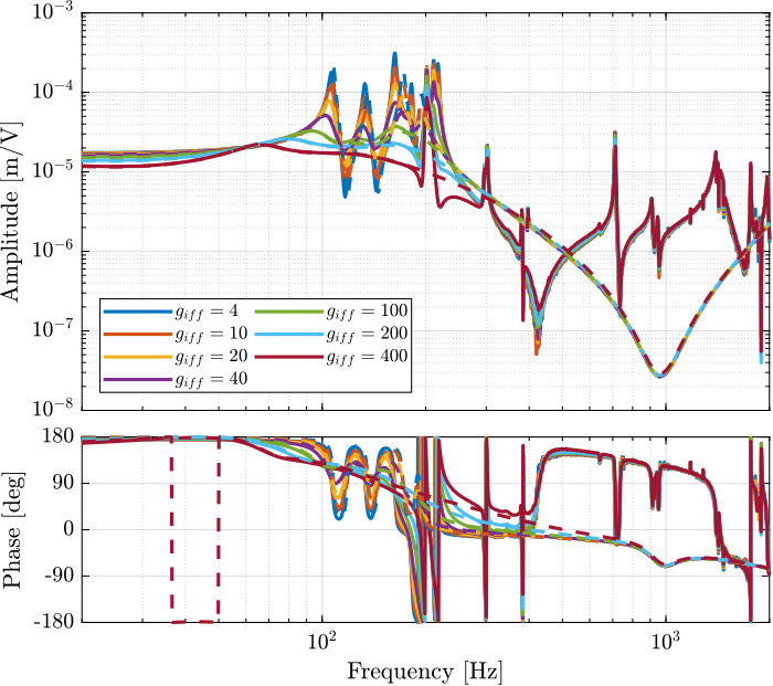
Figure 15: Transfer function from \(u\) to \(d\mathcal{L}_m\) for multiple values of the IFF gain

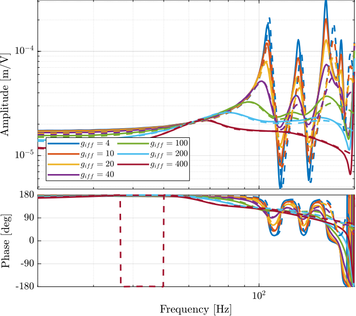
Figure 16: Transfer function from \(u\) to \(d\mathcal{L}_m\) for multiple values of the IFF gain (Zoom)

The IFF control strategy is very effective for the damping of the suspension modes. It however does not damp the modes at 200Hz, 300Hz and 400Hz (flexible modes of the APA). This is very logical.

Also, the experimental results and the models obtained from the Simscape model are in agreement.

1.4.3.4 Experimental Results - Comparison of the un-damped and fully damped system

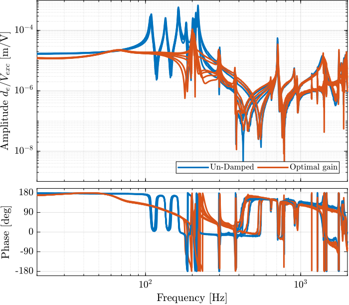
Figure 17: Comparison of the diagonal elements of the tranfer function from \(\bm{u}\) to \(d\bm{\mathcal{L}}_m\) without active damping and with optimal IFF gain

1.4.4 Experimental Results - Damped Plant with Optimal gain

Let’s now look at the \(6 \times 6\) damped plant with the optimal gain \(g = 400\).

1.4.4.1 Load Data

%% Load Identification Data
meas_iff_struts = {};

for i = 1:6
    meas_iff_struts(i) = {load(sprintf('mat/iff_strut_%i_noise_g_400.mat', i), 't', 'Vexc', 'Vs', 'de', 'u')};
end

1.4.4.2 Spectral Analysis - Setup

%% Setup useful variables
% Sampling Time [s]
Ts = (meas_iff_struts{1}.t(end) - (meas_iff_struts{1}.t(1)))/(length(meas_iff_struts{1}.t)-1);

% Sampling Frequency [Hz]
Fs = 1/Ts;

% Hannning Windows
win = hanning(ceil(1*Fs));

% And we get the frequency vector
[~, f] = tfestimate(meas_iff_struts{1}.Vexc, meas_iff_struts{1}.de, win, [], [], 1/Ts);

1.4.4.3 DVF Plant

%% DVF Plant (transfer function from u to dLm)
G_iff_opt = {};

for i = 1:6
    G_iff_opt{i} = tfestimate(meas_iff_struts{i}.Vexc, meas_iff_struts{i}.de, win, [], [], 1/Ts);
end

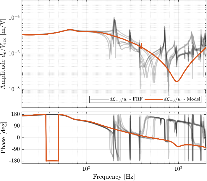
Figure 18: Comparison of the diagonal elements of the transfer functions from \(\bm{u}\) to \(d\bm{\mathcal{L}}_m\) with active damping (IFF) applied with an optimal gain \(g = 400\)

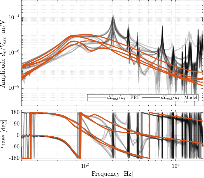
Figure 19: Comparison of the off-diagonal elements of the transfer functions from \(\bm{u}\) to \(d\bm{\mathcal{L}}_m\) with active damping (IFF) applied with an optimal gain \(g = 400\)

With the IFF control strategy applied and the optimal gain used, the suspension modes are very well dapmed. Remains the undamped flexible modes of the APA, and the modes of the plates.

The Simscape model and the experimental results are in very good agreement.

1.5 Modal Analysis

Several 3-axis accelerometers are fixed on the top platform of the nano-hexapod as shown in Figure 22.

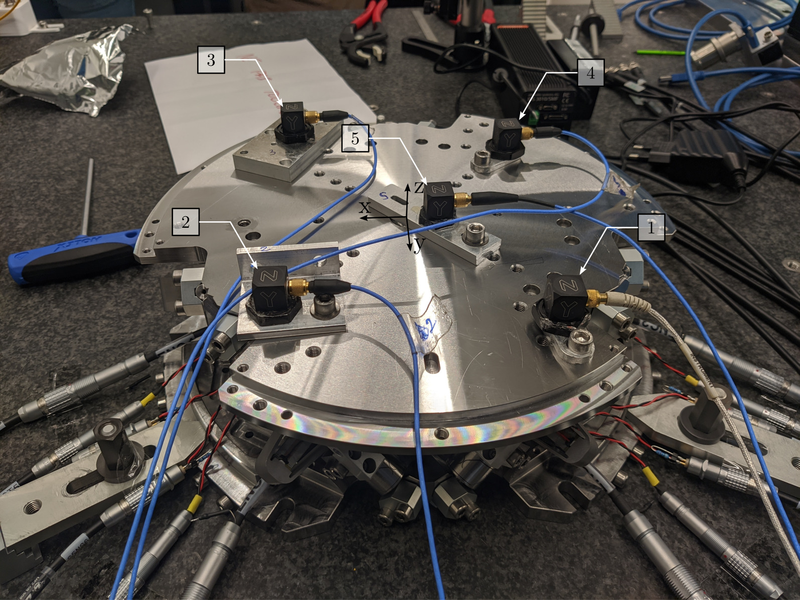
Figure 20: Location of the accelerometers on top of the nano-hexapod

The top platform is then excited using an instrumented hammer as shown in Figure 21.

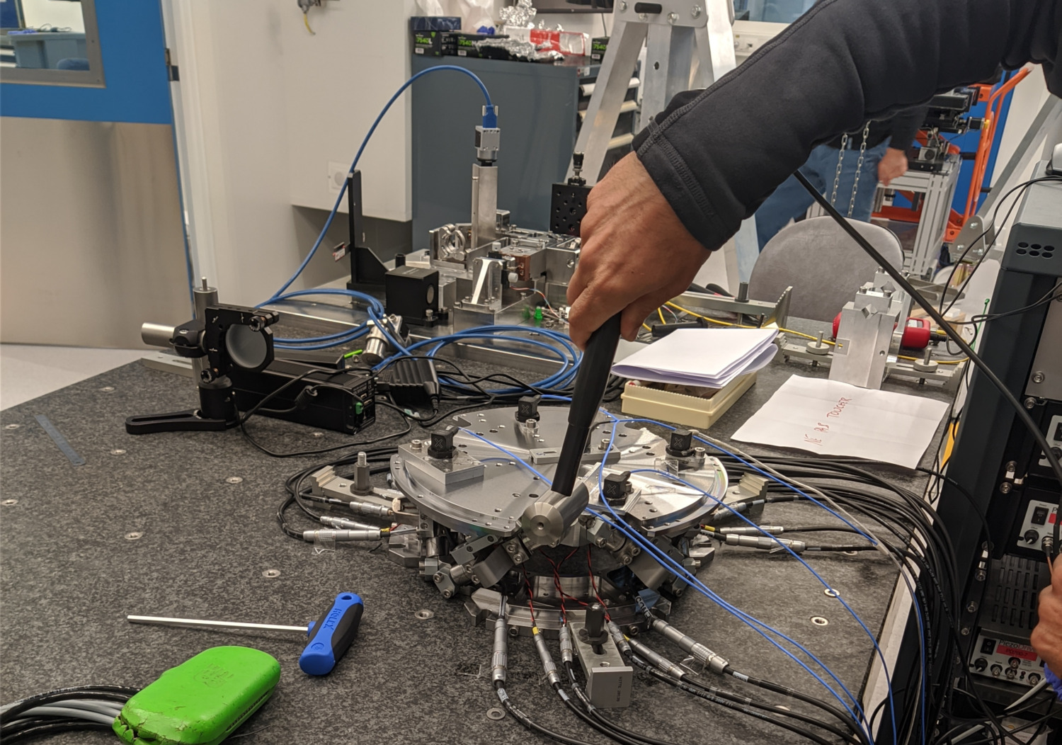
Figure 21: Example of an excitation using an instrumented hammer

1.5.1 Effectiveness of the IFF Strategy - Compliance

In this section, we wish to estimated the effectiveness of the IFF strategy concerning the compliance.

The top plate is excited vertically using the instrumented hammer two times:

no control loop is used
decentralized IFF is used

The data is loaded.

frf_ol  = load('Measurement_Z_axis.mat'); % Open-Loop
frf_iff = load('Measurement_Z_axis_damped.mat'); % IFF

The mean vertical motion of the top platform is computed by averaging all 5 accelerometers.

%% Multiply by 10 (gain in m/s^2/V) and divide by 5 (number of accelerometers)
d_frf_ol = 10/5*(frf_ol.FFT1_H1_4_1_RMS_Y_Mod + frf_ol.FFT1_H1_7_1_RMS_Y_Mod + frf_ol.FFT1_H1_10_1_RMS_Y_Mod + frf_ol.FFT1_H1_13_1_RMS_Y_Mod + frf_ol.FFT1_H1_16_1_RMS_Y_Mod)./(2*pi*frf_ol.FFT1_H1_16_1_RMS_X_Val).^2;
d_frf_iff = 10/5*(frf_iff.FFT1_H1_4_1_RMS_Y_Mod + frf_iff.FFT1_H1_7_1_RMS_Y_Mod + frf_iff.FFT1_H1_10_1_RMS_Y_Mod + frf_iff.FFT1_H1_13_1_RMS_Y_Mod + frf_iff.FFT1_H1_16_1_RMS_Y_Mod)./(2*pi*frf_iff.FFT1_H1_16_1_RMS_X_Val).^2;

The vertical compliance (magnitude of the transfer function from a vertical force applied on the top plate to the vertical motion of the top plate) is shown in Figure 22.

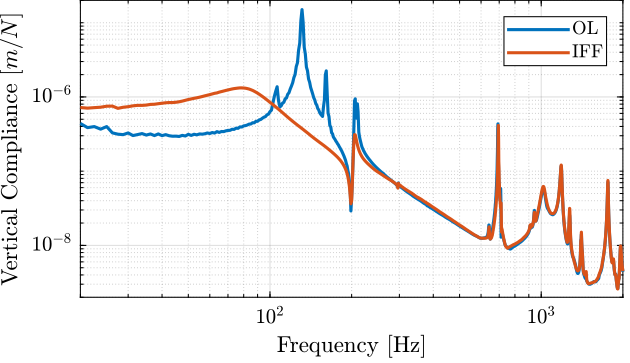
Figure 22: Measured vertical compliance with and without IFF

From Figure 22, it is clear that the IFF control strategy is very effective in damping the suspensions modes of the nano-hexapode. It also has the effect of degrading (slightly) the vertical compliance at low frequency.

1.5.2 Comparison with the Simscape Model

Let’s now compare the measured vertical compliance with the vertical compliance as estimated from the Simscape model.

The transfer function from a vertical external force to the absolute motion of the top platform is identified (with and without IFF) using the Simscape model. The comparison is done in Figure 23. Again, the model is quire accurate!

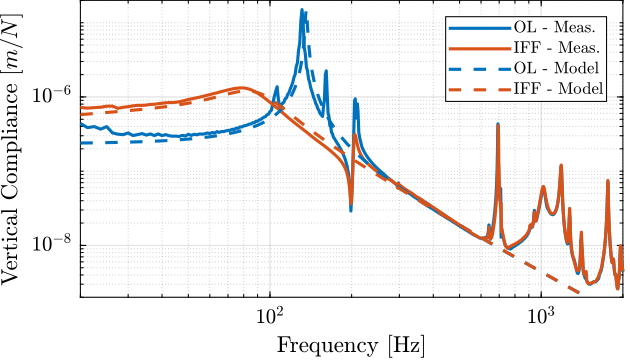
Figure 23: Measured vertical compliance with and without IFF

1.5.3 Obtained Mode Shapes

Then, several excitation are performed using the instrumented Hammer and the mode shapes are extracted.

We can observe the mode shapes of the first 6 modes that are the suspension modes (the plate is behaving as a solid body) in Figure 24.

Figure 24: Measured mode shapes for the first six modes

Then, there is a mode at 692Hz which corresponds to a flexible mode of the top plate (Figure 24).

Figure 25: First flexible mode at 692Hz

The obtained modes are summarized in Table 2.

Table 2: Description of the identified modes
Mode Number	Frequency [Hz]	Description
1	105	Suspension Mode: ~Y-translation
2	107	Suspension Mode: ~X-translation
3	131	Suspension Mode: Z-translation
4	161	Suspension Mode: ~Y-tilt
5	162	Suspension Mode: ~X-tilt
6	180	Suspension Mode: Z-rotation
7	692	(flexible) Membrane mode of the top platform