Nano-Hexapod - Test Bench

1. Encoders fixed to the Struts

This report is also available as a pdf.

Here are the documentation of the equipment used for this test bench:

Voltage Amplifier: PiezoDrive PD200
Amplified Piezoelectric Actuator: Cedrat APA300ML
DAC/ADC: Speedgoat IO313
Encoder: Renishaw Vionic and used Ruler
Interferometers: Attocube

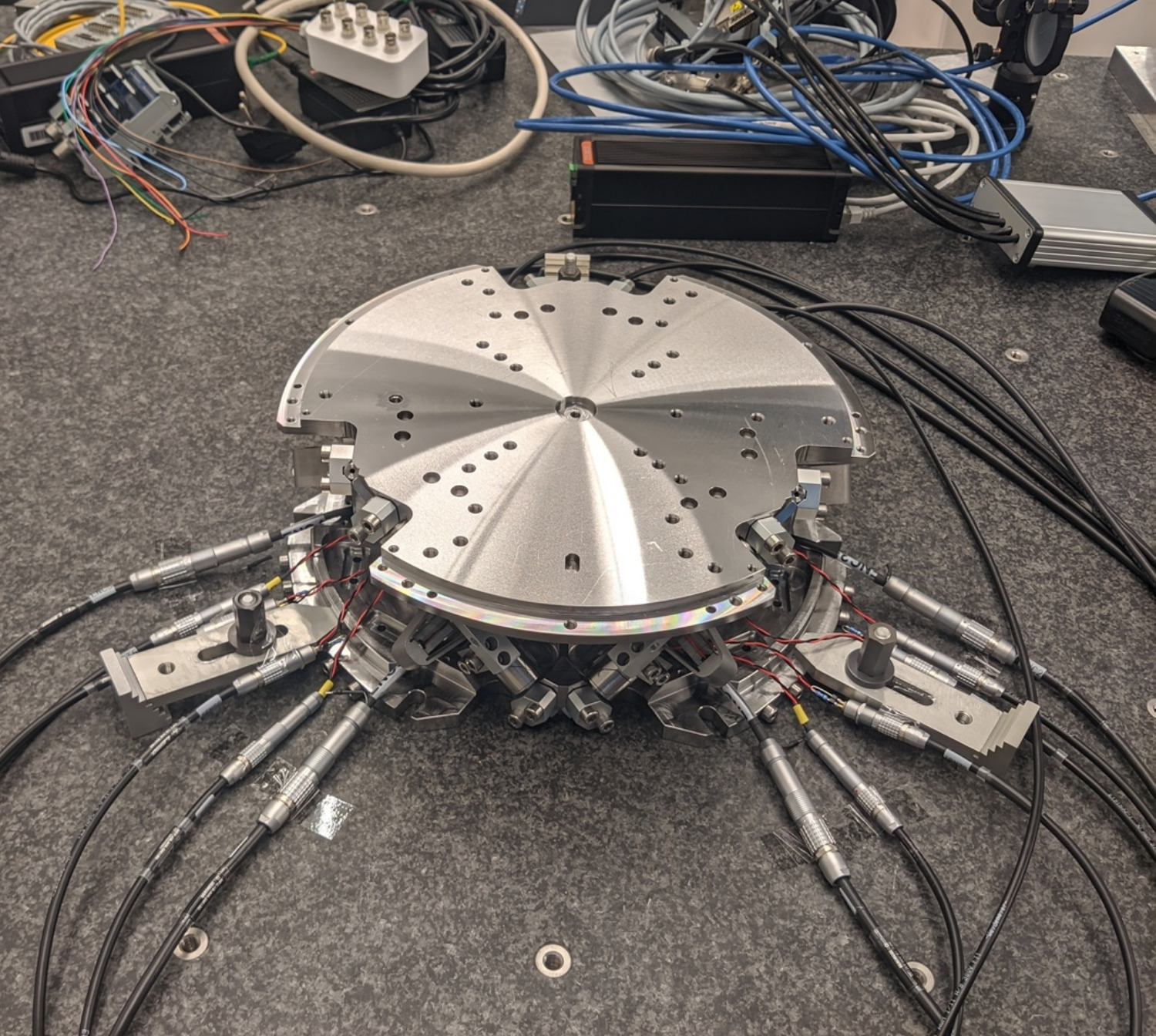
Figure 1: Nano-Hexapod

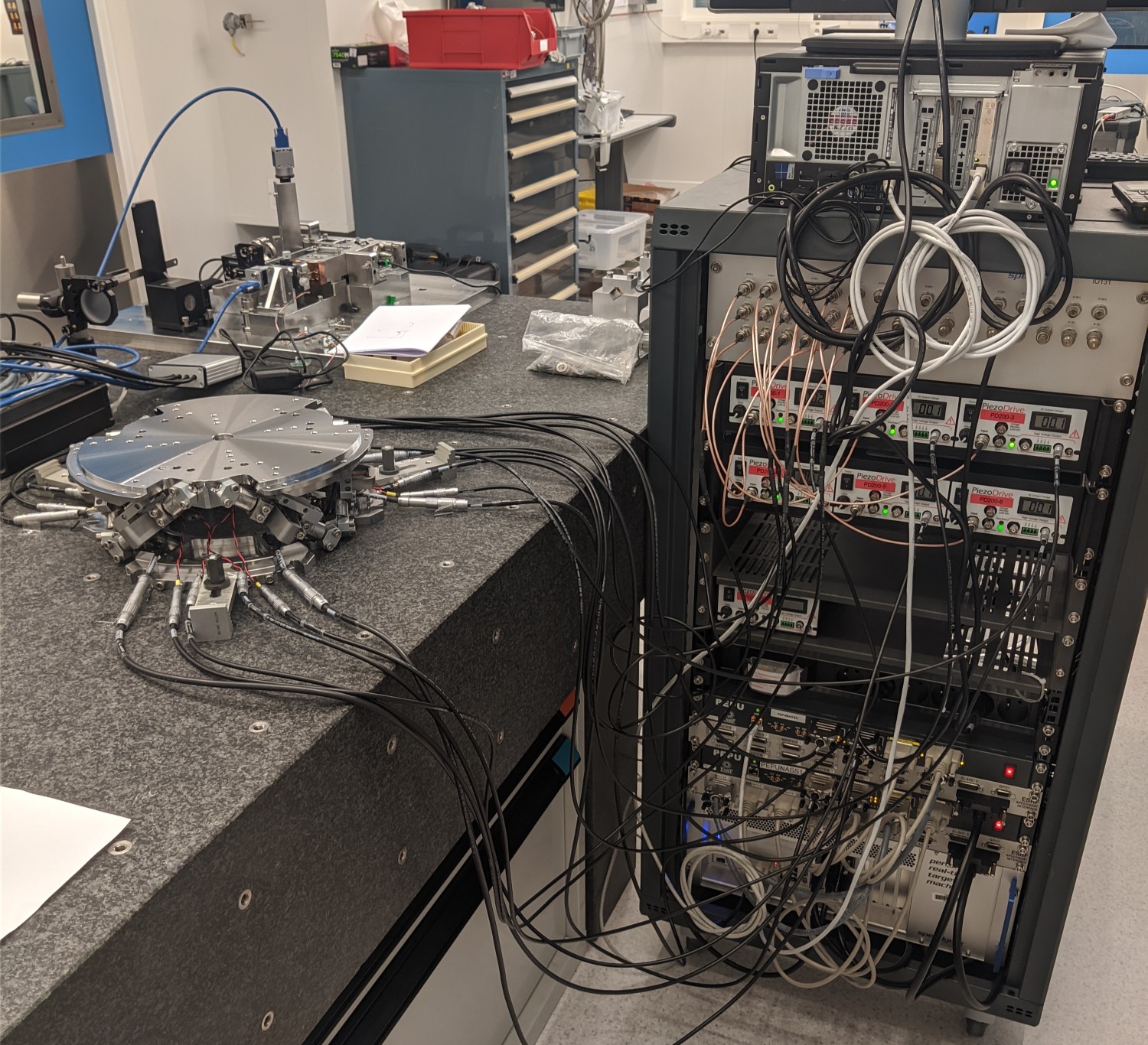
Figure 2: Nano-Hexapod and the control electronics

1 Encoders fixed to the Struts

1.1 Introduction

1.2 Load Data

meas_data_lf = {};

for i = 1:6
    meas_data_lf(i) = {load(sprintf('mat/frf_data_exc_strut_%i_noise_lf.mat', i), 't', 'Va', 'Vs', 'de')};
    meas_data_hf(i) = {load(sprintf('mat/frf_data_exc_strut_%i_noise_hf.mat', i), 't', 'Va', 'Vs', 'de')};
end

1.3 Spectral Analysis - Setup

% Sampling Time [s]
Ts = (meas_data_lf{1}.t(end) - (meas_data_lf{1}.t(1)))/(length(meas_data_lf{1}.t)-1);

% Sampling Frequency [Hz]
Fs = 1/Ts;

% Hannning Windows
win = hanning(ceil(1*Fs));

And we get the frequency vector.

[~, f] = tfestimate(meas_data_lf{1}.Va, meas_data_lf{1}.de, win, [], [], 1/Ts);

i_lf = f < 250; % Points for low frequency excitation
i_hf = f > 250; % Points for high frequency excitation

1.4 DVF Plant

First, let’s compute the coherence from the excitation voltage and the displacement as measured by the encoders (Figure 3).

%% Coherence
coh_dvf_lf = zeros(length(f), 6, 6);
coh_dvf_hf = zeros(length(f), 6, 6);

for i = 1:6
    coh_dvf_lf(:, :, i) = mscohere(meas_data_lf{i}.Va, meas_data_lf{i}.de, win, [], [], 1/Ts);
    coh_dvf_hf(:, :, i) = mscohere(meas_data_hf{i}.Va, meas_data_hf{i}.de, win, [], [], 1/Ts);
end

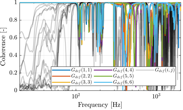
Figure 3: Obtained coherence for the DVF plant

Then the 6x6 transfer function matrix is estimated (Figure 4).

%% DVF Plant
G_dvf_lf = zeros(length(f), 6, 6);
G_dvf_hf = zeros(length(f), 6, 6);

for i = 1:6
    G_dvf_lf(:, :, i) = tfestimate(meas_data_lf{i}.Va, meas_data_lf{i}.de, win, [], [], 1/Ts);
    G_dvf_hf(:, :, i) = tfestimate(meas_data_hf{i}.Va, meas_data_hf{i}.de, win, [], [], 1/Ts);
end

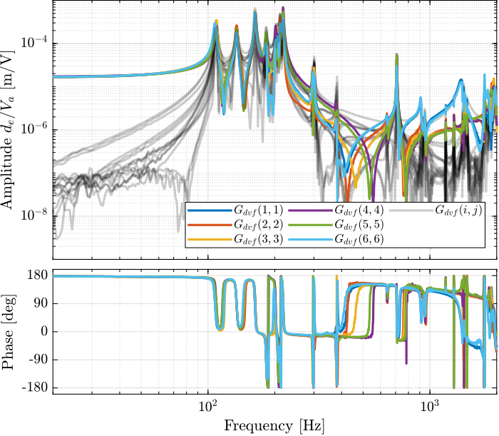
Figure 4: Measured FRF for the DVF plant

1.5 IFF Plant

First, let’s compute the coherence from the excitation voltage and the displacement as measured by the encoders (Figure 5).

%% Coherence
coh_iff_lf = zeros(length(f), 6, 6);
coh_iff_hf = zeros(length(f), 6, 6);

for i = 1:6
    coh_iff_lf(:, :, i) = mscohere(meas_data_lf{i}.Va, meas_data_lf{i}.Vs, win, [], [], 1/Ts);
    coh_iff_hf(:, :, i) = mscohere(meas_data_hf{i}.Va, meas_data_hf{i}.Vs, win, [], [], 1/Ts);
end

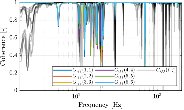
Figure 5: Obtained coherence for the IFF plant

Then the 6x6 transfer function matrix is estimated (Figure 6).

%% IFF Plant
G_iff_lf = zeros(length(f), 6, 6);
G_iff_hf = zeros(length(f), 6, 6);

for i = 1:6
    G_iff_lf(:, :, i) = tfestimate(meas_data_lf{i}.Va, meas_data_lf{i}.Vs, win, [], [], 1/Ts);
    G_iff_hf(:, :, i) = tfestimate(meas_data_hf{i}.Va, meas_data_hf{i}.Vs, win, [], [], 1/Ts);
end

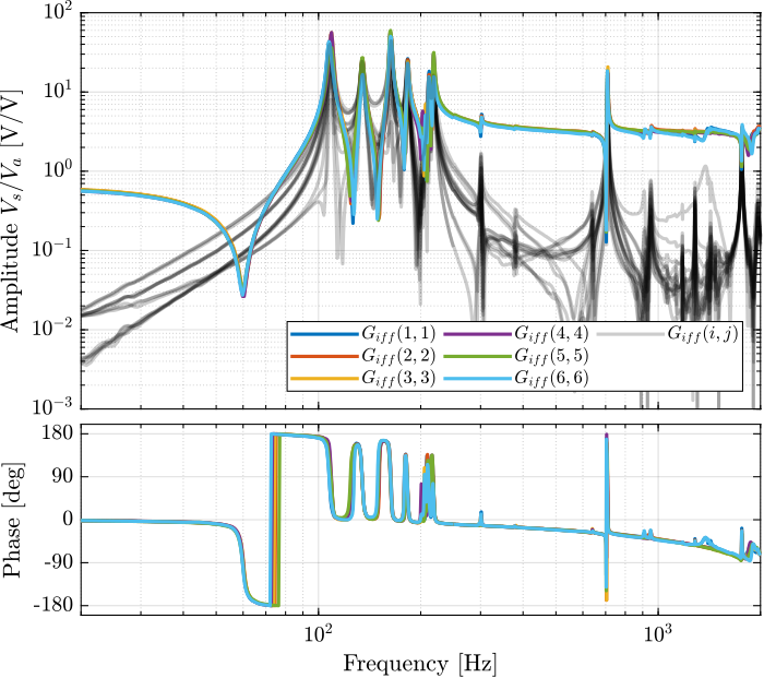
Figure 6: Measured FRF for the IFF plant

1.6 Jacobian

load('jacobian.mat', 'J');

1.6.1 DVF Plant

G_dvf_J_lf = permute(pagemtimes(inv(J), pagemtimes(permute(G_dvf_lf, [2 3 1]), inv(J'))), [3 1 2]);
G_dvf_J_hf = permute(pagemtimes(inv(J), pagemtimes(permute(G_dvf_hf, [2 3 1]), inv(J'))), [3 1 2]);

1.6.2 IFF Plant

G_iff_J_lf = permute(pagemtimes(inv(J), pagemtimes(permute(G_iff_lf, [2 3 1]), inv(J'))), [3 1 2]);
G_iff_J_hf = permute(pagemtimes(inv(J), pagemtimes(permute(G_iff_hf, [2 3 1]), inv(J'))), [3 1 2]);