Nano-Hexapod - Test Bench

1. Encoders fixed to the Struts
2. Encoders fixed to the plates

This report is also available as a pdf.

In this document, the dynamics of the nano-hexapod shown in Figure 1 is identified.

Here are the documentation of the equipment used for this test bench:

Voltage Amplifier: PiezoDrive PD200
Amplified Piezoelectric Actuator: Cedrat APA300ML
DAC/ADC: Speedgoat IO313
Encoder: Renishaw Vionic and used Ruler
Interferometers: Attocube

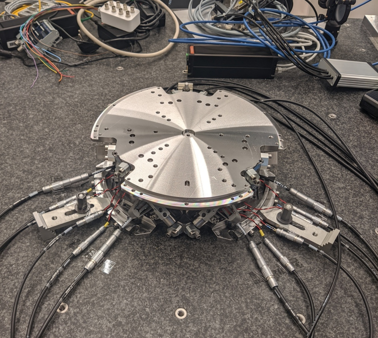
Figure 1: Nano-Hexapod

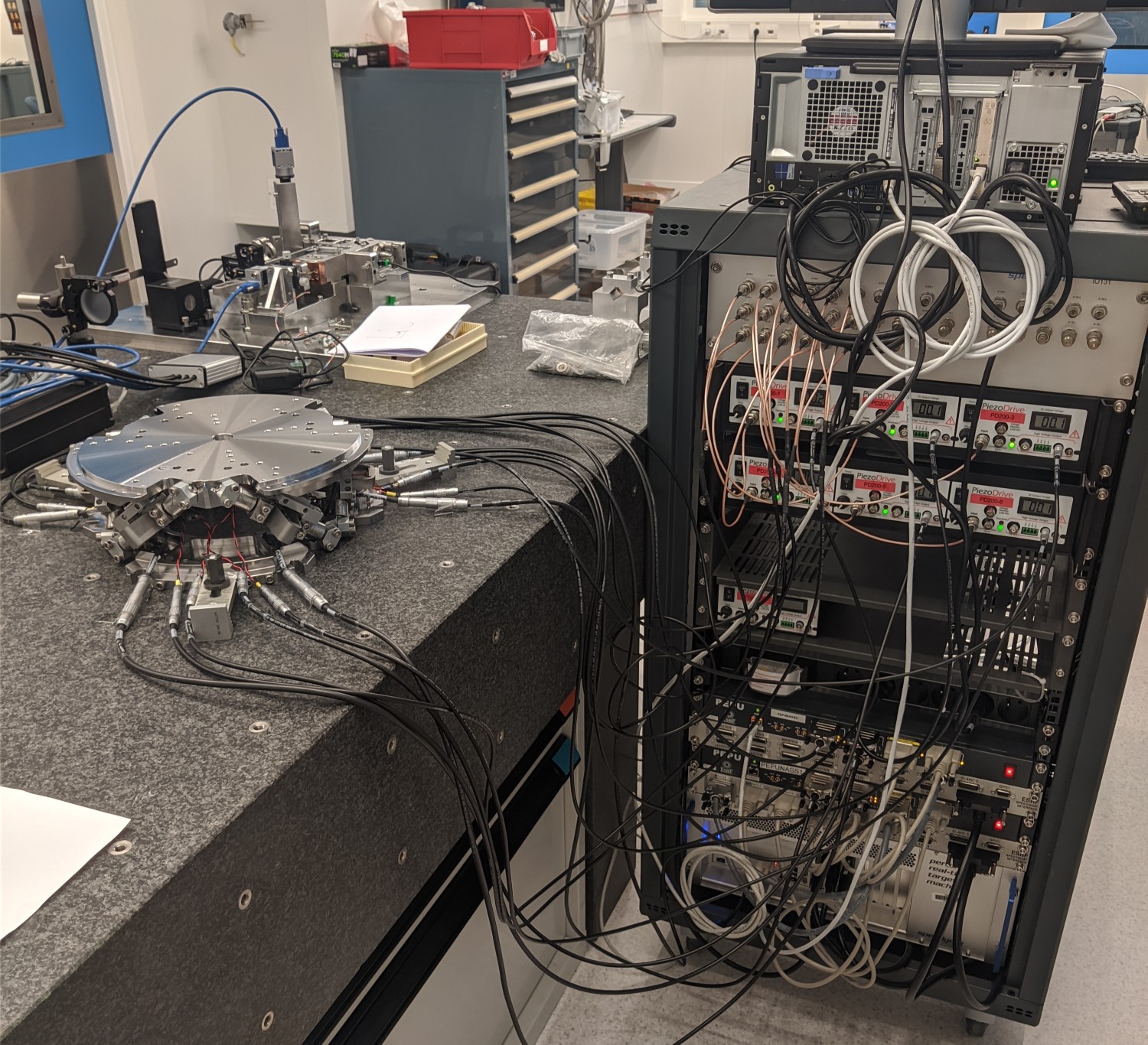
Figure 2: Nano-Hexapod and the control electronics

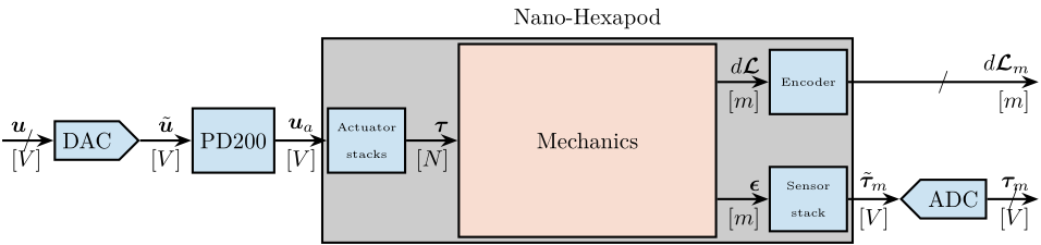
Figure 3: Block diagram of the system with named signals

Table 1: List of signals
	Unit	Matlab	Vector	Elements
Control Input (wanted DAC voltage)	`[V]`	`u`	\(\bm{u}\)	\(u_i\)
DAC Output Voltage	`[V]`	`u`	\(\tilde{\bm{u}}\)	\(\tilde{u}_i\)
PD200 Output Voltage	`[V]`	`ua`	\(\bm{u}_a\)	\(u_{a,i}\)
Actuator applied force	`[N]`	`tau`	\(\bm{\tau}\)	\(\tau_i\)
Strut motion	`[m]`	`dL`	\(d\bm{\mathcal{L}}\)	\(d\mathcal{L}_i\)
Encoder measured displacement	`[m]`	`dLm`	\(d\bm{\mathcal{L}}_m\)	\(d\mathcal{L}_{m,i}\)
Force Sensor strain	`[m]`	`epsilon`	\(\bm{\epsilon}\)	\(\epsilon_i\)
Force Sensor Generated Voltage	`[V]`	`taum`	\(\tilde{\bm{\tau}}_m\)	\(\tilde{\tau}_{m,i}\)
Measured Generated Voltage	`[V]`	`taum`	\(\bm{\tau}_m\)	\(\tau_{m,i}\)
Motion of the top platform	`[m,rad]`	`dX`	\(d\bm{\mathcal{X}}\)	\(d\mathcal{X}_i\)
Metrology measured displacement	`[m,rad]`	`dXm`	\(d\bm{\mathcal{X}}_m\)	\(d\mathcal{X}_{m,i}\)

1 Encoders fixed to the Struts

1.1 Introduction

In this section, the encoders are fixed to the struts.

1.2 Identification of the dynamics

1.2.1 Load Data

%% Load Identification Data
meas_data_lf = {};

for i = 1:6
    meas_data_lf(i) = {load(sprintf('mat/frf_data_exc_strut_%i_noise_lf.mat', i), 't', 'Va', 'Vs', 'de')};
    meas_data_hf(i) = {load(sprintf('mat/frf_data_exc_strut_%i_noise_hf.mat', i), 't', 'Va', 'Vs', 'de')};
end

1.2.2 Spectral Analysis - Setup

%% Setup useful variables
% Sampling Time [s]
Ts = (meas_data_lf{1}.t(end) - (meas_data_lf{1}.t(1)))/(length(meas_data_lf{1}.t)-1);

% Sampling Frequency [Hz]
Fs = 1/Ts;

% Hannning Windows
win = hanning(ceil(1*Fs));

% And we get the frequency vector
[~, f] = tfestimate(meas_data_lf{1}.Va, meas_data_lf{1}.de, win, [], [], 1/Ts);

i_lf = f < 250; % Points for low frequency excitation
i_hf = f > 250; % Points for high frequency excitation

1.2.3 DVF Plant

First, let’s compute the coherence from the excitation voltage and the displacement as measured by the encoders (Figure 4).

%% Coherence
coh_dvf_lf = zeros(length(f), 6, 6);
coh_dvf_hf = zeros(length(f), 6, 6);

for i = 1:6
    coh_dvf_lf(:, :, i) = mscohere(meas_data_lf{i}.Va, meas_data_lf{i}.de, win, [], [], 1/Ts);
    coh_dvf_hf(:, :, i) = mscohere(meas_data_hf{i}.Va, meas_data_hf{i}.de, win, [], [], 1/Ts);
end

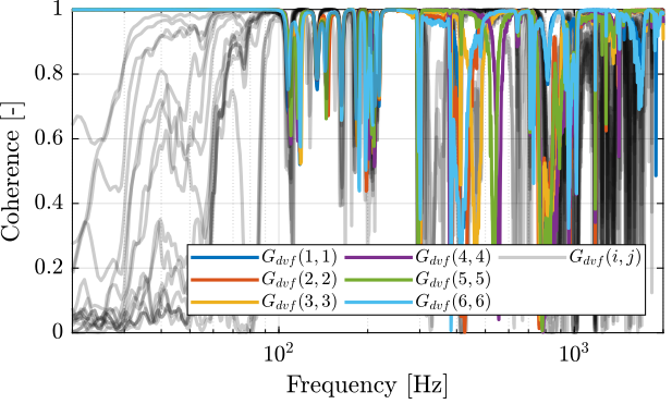
Figure 4: Obtained coherence for the DVF plant

Then the 6x6 transfer function matrix is estimated (Figure 5).

%% DVF Plant (transfer function from u to dLm)
G_dvf_lf = zeros(length(f), 6, 6);
G_dvf_hf = zeros(length(f), 6, 6);

for i = 1:6
    G_dvf_lf(:, :, i) = tfestimate(meas_data_lf{i}.Va, meas_data_lf{i}.de, win, [], [], 1/Ts);
    G_dvf_hf(:, :, i) = tfestimate(meas_data_hf{i}.Va, meas_data_hf{i}.de, win, [], [], 1/Ts);
end

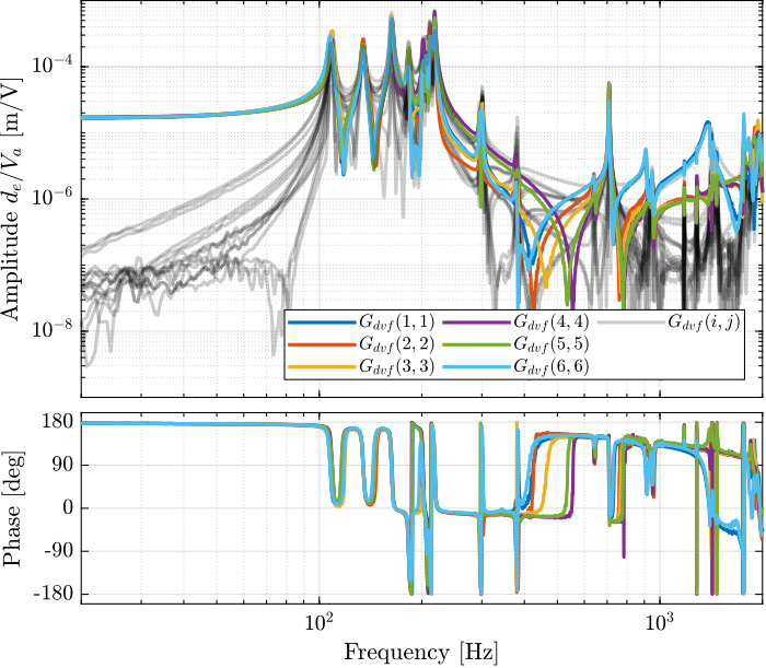
Figure 5: Measured FRF for the DVF plant

1.2.4 IFF Plant

First, let’s compute the coherence from the excitation voltage and the displacement as measured by the encoders (Figure 6).

%% Coherence for the IFF plant
coh_iff_lf = zeros(length(f), 6, 6);
coh_iff_hf = zeros(length(f), 6, 6);

for i = 1:6
    coh_iff_lf(:, :, i) = mscohere(meas_data_lf{i}.Va, meas_data_lf{i}.Vs, win, [], [], 1/Ts);
    coh_iff_hf(:, :, i) = mscohere(meas_data_hf{i}.Va, meas_data_hf{i}.Vs, win, [], [], 1/Ts);
end

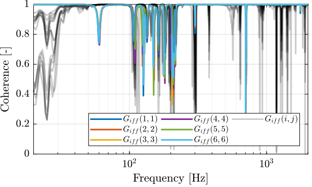
Figure 6: Obtained coherence for the IFF plant

Then the 6x6 transfer function matrix is estimated (Figure 7).

%% IFF Plant
G_iff_lf = zeros(length(f), 6, 6);
G_iff_hf = zeros(length(f), 6, 6);

for i = 1:6
    G_iff_lf(:, :, i) = tfestimate(meas_data_lf{i}.Va, meas_data_lf{i}.Vs, win, [], [], 1/Ts);
    G_iff_hf(:, :, i) = tfestimate(meas_data_hf{i}.Va, meas_data_hf{i}.Vs, win, [], [], 1/Ts);
end

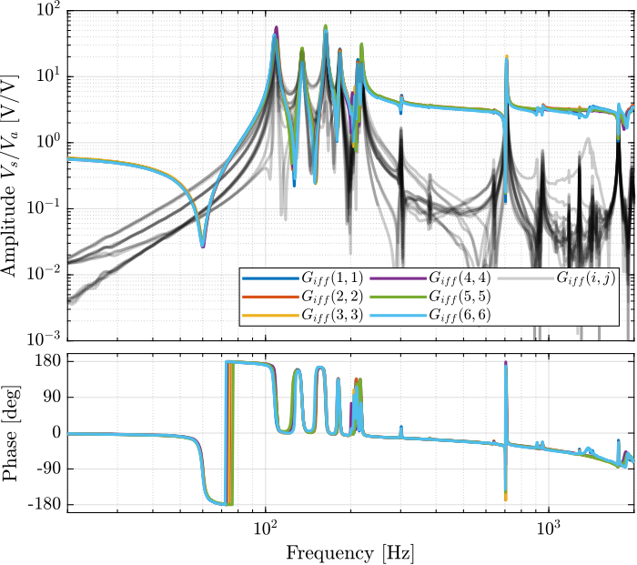
Figure 7: Measured FRF for the IFF plant

1.3 Comparison with the Simscape Model

In this section, the measured dynamics is compared with the dynamics estimated from the Simscape model.

1.3.1 Dynamics from Actuator to Force Sensors

%% Initialize Nano-Hexapod
n_hexapod = initializeNanoHexapodFinal('flex_bot_type', '4dof', ...
                                       'flex_top_type', '4dof', ...
                                       'motion_sensor_type', 'struts', ...
                                       'actuator_type', '2dof');

%% Identify the IFF Plant (transfer function from u to taum)
clear io; io_i = 1;
io(io_i) = linio([mdl, '/F'],  1, 'openinput');   io_i = io_i + 1; % Actuator Inputs
io(io_i) = linio([mdl, '/Fm'],  1, 'openoutput'); io_i = io_i + 1; % Force Sensors

Giff = exp(-s*Ts)*linearize(mdl, io, 0.0, options);

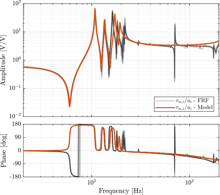
Figure 8: Diagonal elements of the IFF Plant

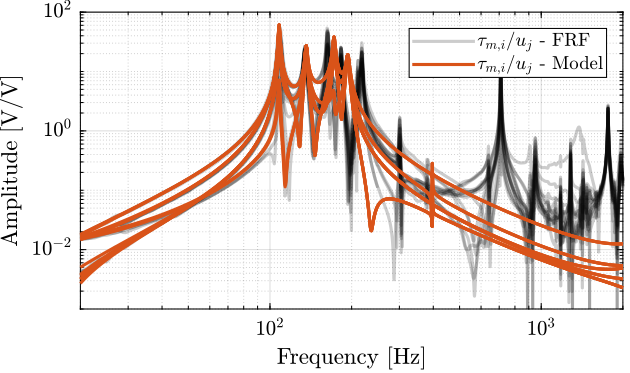
Figure 9: Off diagonal elements of the IFF Plant

1.3.2 Dynamics from Actuator to Encoder

%% Initialization of the Nano-Hexapod
n_hexapod = initializeNanoHexapodFinal('flex_bot_type', '4dof', ...
                                       'flex_top_type', '4dof', ...
                                       'motion_sensor_type', 'struts', ...
                                       'actuator_type', '2dof');

%% Identify the DVF Plant (transfer function from u to dLm)
clear io; io_i = 1;
io(io_i) = linio([mdl, '/F'],  1, 'openinput');  io_i = io_i + 1; % Actuator Inputs
io(io_i) = linio([mdl, '/D'],  1, 'openoutput'); io_i = io_i + 1; % Encoders

Gdvf = exp(-s*Ts)*linearize(mdl, io, 0.0, options);

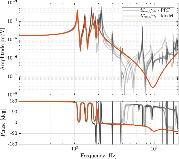
Figure 10: Diagonal elements of the DVF Plant

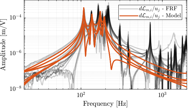
Figure 11: Off diagonal elements of the DVF Plant

1.4 Integral Force Feedback

1.4.1 Root Locus and Decentralized Loop gain

%% IFF Controller
Kiff_g1 = (1/(s + 2*pi*40))*... % Low pass filter (provides integral action above 40Hz)
          (s/(s + 2*pi*30))*... % High pass filter to limit low frequency gain
          (1/(1 + s/2/pi/500))*... % Low pass filter to be more robust to high frequency resonances
          eye(6); % Diagonal 6x6 controller

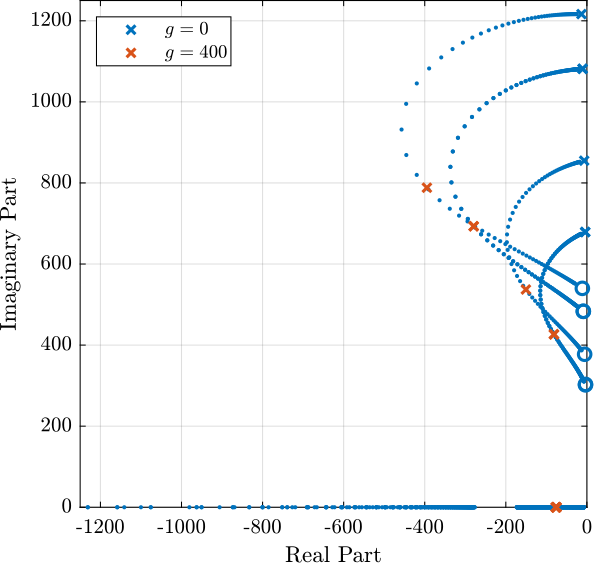
Figure 12: Root Locus for the IFF control strategy

Then the “optimal” IFF controller is:

%% IFF controller with Optimal gain
Kiff = g*Kiff_g1;

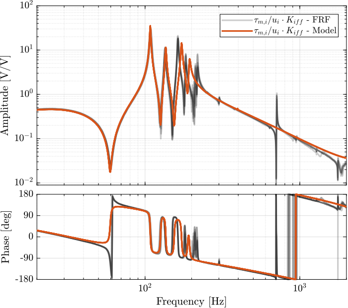
Figure 13: Bode plot of the “decentralized loop gain” \(G_\text{iff}(i,i) \times K_\text{iff}(i,i)\)

1.4.2 Multiple Gains - Simulation

%% Tested IFF gains
iff_gains = [4, 10, 20, 40, 100, 200, 400, 1000];

%% Initialize the Simscape model in closed loop
n_hexapod = initializeNanoHexapodFinal('flex_bot_type', '4dof', ...
                                       'flex_top_type', '4dof', ...
                                       'motion_sensor_type', 'struts', ...
                                       'actuator_type', '2dof', ...
                                       'controller_type', 'iff');

%% Identify the (damped) transfer function from u to dLm for different values of the IFF gain
Gd_iff = {zeros(1, length(iff_gains))};

clear io; io_i = 1;
io(io_i) = linio([mdl, '/F'],  1, 'openinput');  io_i = io_i + 1; % Actuator Inputs
io(io_i) = linio([mdl, '/D'],  1, 'openoutput'); io_i = io_i + 1; % Strut Displacement (encoder)

for i = 1:length(iff_gains)
    Kiff = iff_gains(i)*Kiff_g1*eye(6); % IFF Controller
    Gd_iff(i) = {exp(-s*Ts)*linearize(mdl, io, 0.0, options)};

    isstable(Gd_iff{i})
end

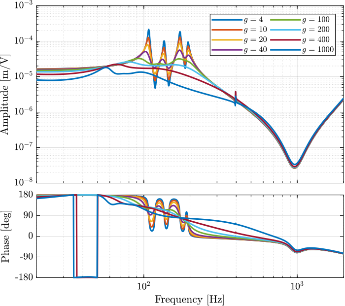
Figure 14: Effect of the IFF gain \(g\) on the transfer function from \(\bm{\tau}\) to \(d\bm{\mathcal{L}}_m\)