Piezoelectric Force Sensor - Test Bench
Table of Contents
In this document is studied how a piezoelectric stack can be used to measured the force.
- Section 1: the effect of the input impedance of the electronics connected to the force sensor stack on the stiffness of the stack is studied
- Section 2:
1 Change of Stiffness due to Sensors stack being open/closed circuit
1.1 Load Data
oc = load('identification_open_circuit.mat', 't', 'encoder', 'u');
sc = load('identification_short_circuit.mat', 't', 'encoder', 'u');
1.2 Transfer Functions
Ts = 1e-4; % Sampling Time [s]
win = hann(ceil(10/Ts));
[tf_oc_est, f] = tfestimate(oc.u, oc.encoder, win, [], [], 1/Ts);
[co_oc_est, ~] = mscohere(  oc.u, oc.encoder, win, [], [], 1/Ts);

[tf_sc_est, ~] = tfestimate(sc.u, sc.encoder, win, [], [], 1/Ts);
[co_sc_est, ~] = mscohere(  sc.u, sc.encoder, win, [], [], 1/Ts);
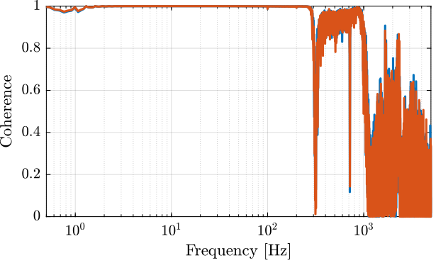
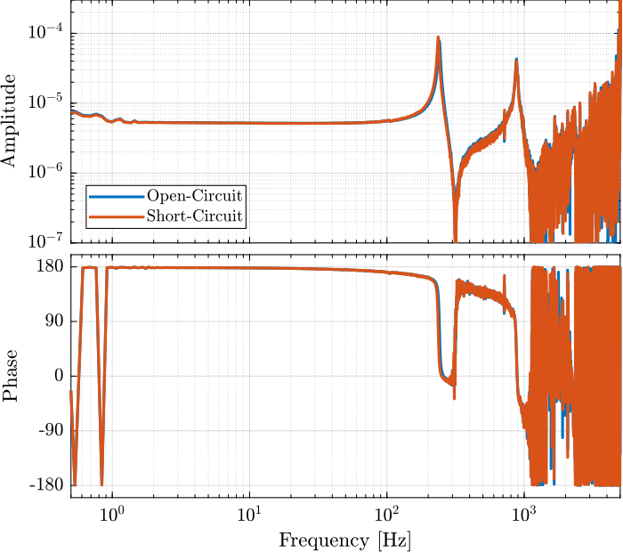
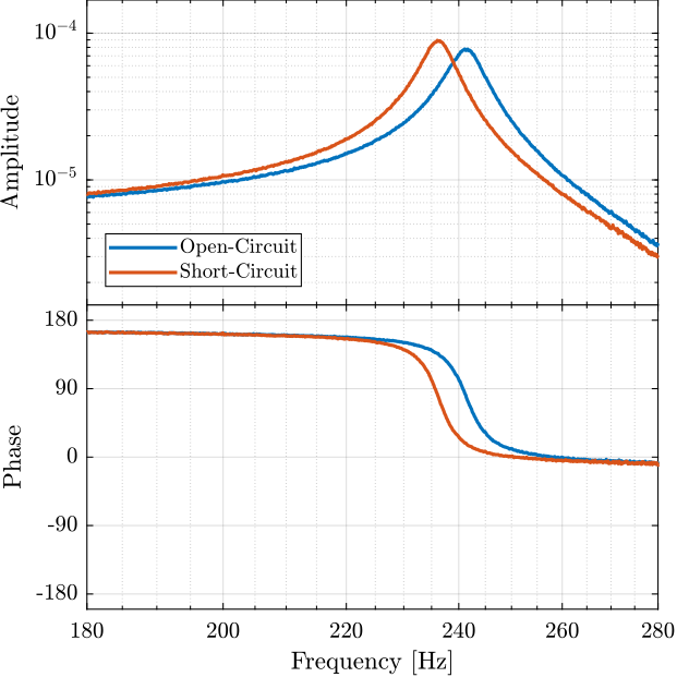
Figure 3: Zoom on the change of resonance
The change of resonance frequency / stiffness is very small and is not important here.
2 Generated Number of Charge / Voltage
Two stacks are used as actuator (in parallel) and one stack is used as sensor.
The amplifier gain is 20V/V (Cedrat LA75B).
2.1 Steps
load('force_sensor_steps.mat', 't', 'encoder', 'u', 'v');
figure;
tiledlayout(2, 1, 'TileSpacing', 'None', 'Padding', 'None');
nexttile;
plot(t, v);
xlabel('Time [s]'); ylabel('Measured voltage [V]');
nexttile;
plot(t, u);
xlabel('Time [s]'); ylabel('Actuator Voltage [V]');
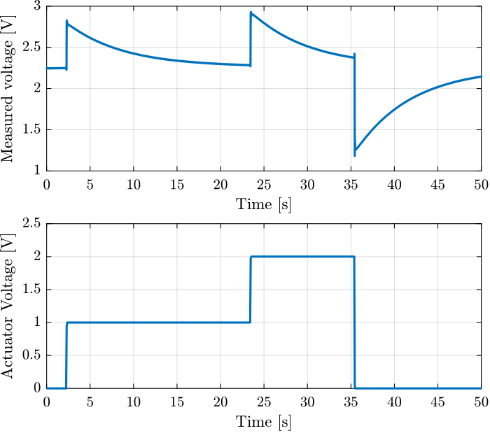
Figure 4: Time domain signal during the 3 actuator voltage steps
Three steps are performed at the following time intervals:
t_s = [ 2.5, 23;
       23.8, 35;
       35.8, 50];
Fit function:
f = @(b,x) b(1).*exp(b(2).*x) + b(3);
We are interested by the b(2) term, which is the time constant of the exponential.
tau = zeros(size(t_s, 1),1);
V0  = zeros(size(t_s, 1),1);
for t_i = 1:size(t_s, 1)
    t_cur = t(t_s(t_i, 1) < t & t < t_s(t_i, 2));
    t_cur = t_cur - t_cur(1);
    y_cur = v(t_s(t_i, 1) < t & t < t_s(t_i, 2));

    nrmrsd = @(b) norm(y_cur - f(b,t_cur)); % Residual Norm Cost Function
    B0 = [0.5, -0.15, 2.2];                        % Choose Appropriate Initial Estimates
    [B,rnrm] = fminsearch(nrmrsd, B0);     % Estimate Parameters ‘B’

    tau(t_i) = 1/B(2);
    V0(t_i)  = B(3);
end
| \(tau\) [s] | \(V_0\) [V] |
|---|---|
| 6.47 | 2.26 |
| 6.76 | 2.26 |
| 6.49 | 2.25 |
With the capacitance being \(C = 4.4 \mu F\), the internal impedance of the Speedgoat ADC can be computed as follows:
Cp = 4.4e-6; % [F]
Rin = abs(mean(tau))/Cp;
1494100.0
The input impedance of the Speedgoat’s ADC should then be close to \(1.5\,M\Omega\) (specified at \(1\,M\Omega\)).
How can we explain the voltage offset?
As shown in Figure 5 (taken from (Reza and Andrew 2006)), an input voltage offset is due to the input bias current \(i_n\).
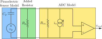
Figure 5: Model of a piezoelectric transducer (left) and instrumentation amplifier (right)
The estimated input bias current is then:
in = mean(V0)/Rin;
1.5119e-06
An additional resistor in parallel with \(R_{in}\) would have two effects:
- reduce the input voltage offset \[ V_{off} = \frac{R_a R_{in}}{R_a + R_{in}} i_n \]
- increase the high pass corner frequency \(f_c\) \[ C_p \frac{R_{in}R_a}{R_{in} + R_a} = \tau_c = \frac{1}{f_c} \] \[ R_a = \frac{R_i}{f_c C_p R_i - 1} \]
If we allow the high pass corner frequency to be equals to 3Hz:
fc = 3;
Ra = Rin/(fc*Cp*Rin - 1);
79804
With this parallel resistance value, the voltage offset would be:
V_offset = Ra*Rin/(Ra + Rin) * in;
0.11454
Which is much more acceptable.
2.2 Add Parallel Resistor
A resistor \(R_p \approx 100\,k\Omega\) is added in parallel with the force sensor as shown in Figure 6.
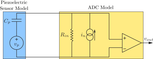
Figure 6: Model of a piezoelectric transducer (left) and instrumentation amplifier (right) with added resistor \(R_p\)
load('force_sensor_steps_R_82k7.mat', 't', 'encoder', 'u', 'v');
figure;
tiledlayout(2, 1, 'TileSpacing', 'None', 'Padding', 'None');
nexttile;
plot(t, v);
xlabel('Time [s]'); ylabel('Measured voltage [V]');
nexttile;
plot(t, u);
xlabel('Time [s]'); ylabel('Actuator Voltage [V]');
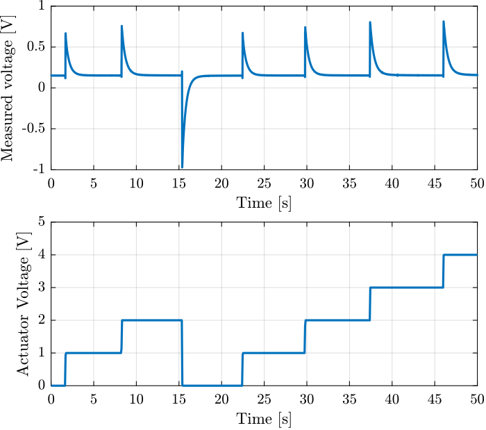
Figure 7: Time domain signal during the actuator voltage steps
Three steps are performed at the following time intervals:
t_s = [1.9,  6;
       8.5, 13;
      15.5, 21;
      22.6, 26;
      30.0, 36;
      37.5, 41;
      46.2, 49.5]
Fit function:
f = @(b,x) b(1).*exp(b(2).*x) + b(3);
We are interested by the b(2) term, which is the time constant of the exponential.
tau = zeros(size(t_s, 1),1);
V0  = zeros(size(t_s, 1),1);
for t_i = 1:size(t_s, 1)
    t_cur = t(t_s(t_i, 1) < t & t < t_s(t_i, 2));
    t_cur = t_cur - t_cur(1);
    y_cur = v(t_s(t_i, 1) < t & t < t_s(t_i, 2));

    nrmrsd = @(b) norm(y_cur - f(b,t_cur)); % Residual Norm Cost Function
    B0 = [0.5, -0.2, 0.2];                        % Choose Appropriate Initial Estimates
    [B,rnrm] = fminsearch(nrmrsd, B0);     % Estimate Parameters ‘B’

    tau(t_i) = 1/B(2);
    V0(t_i)  = B(3);
end
And indeed, we obtain a much smaller offset voltage and a much faster time constant.
| \(tau\) [s] | \(V_0\) [V] |
|---|---|
| 0.43 | 0.15 |
| 0.45 | 0.16 |
| 0.43 | 0.15 |
| 0.43 | 0.15 |
| 0.45 | 0.15 |
| 0.46 | 0.16 |
| 0.48 | 0.16 |
Knowing the capacitance value, we can estimate the value of the added resistor (neglecting the input impedance of \(\approx 1\,M\Omega\)):
Cp = 4.4e-6; % [F]
Rin = abs(mean(tau))/Cp;
101200.0
And we can verify that the bias current estimation stays the same:
in = mean(V0)/Rin;
1.5305e-06
This validates the model of the ADC and the effectiveness of the added resistor.
2.3 Sinus
load('force_sensor_sin.mat', 't', 'encoder', 'u', 'v');

u       = u(t>25);
v       = v(t>25);
encoder = encoder(t>25) - mean(encoder(t>25));
t       = t(t>25);
The driving voltage is a sinus at 0.5Hz centered on 3V and with an amplitude of 3V (Figure 8).
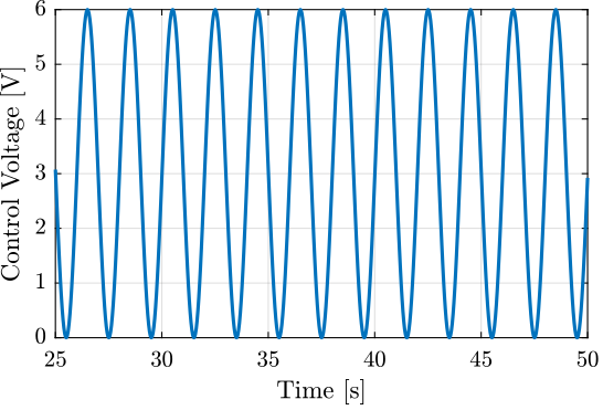
Figure 8: Driving Voltage
The full stroke as measured by the encoder is:
max(encoder)-min(encoder)
5.005e-05
Its signal is shown in Figure 9.
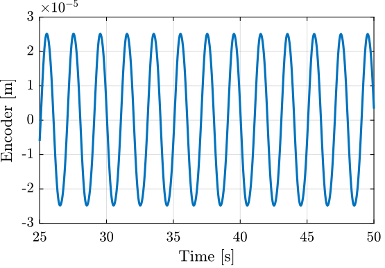
Figure 9: Encoder measurement
The generated voltage by the stack is shown in Figure
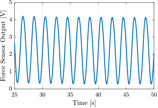
Figure 10: Voltage measured on the stack used as a sensor
The capacitance of the stack is
Cp = 4.4e-6; % [F]
The corresponding generated charge is then shown in Figure 11.
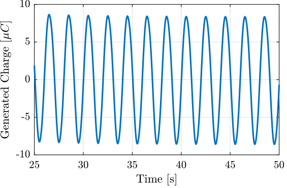
Figure 11: Generated Charge
The relation between the generated voltage and the measured displacement is almost linear as shown in Figure 12.
b1 = encoder\(v-mean(v));
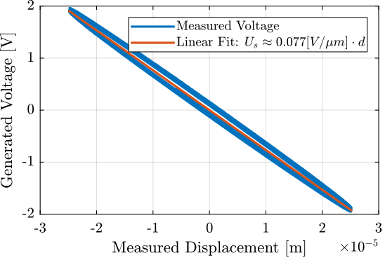
Figure 12: Almost linear relation between the relative displacement and the generated voltage
With a 16bits ADC, the resolution will then be equals to (in [nm]):
abs((20/2^16)/(b1/1e9))
3.9838