Flexible Joint - Test Bench

1. Finite Element Model
- 1.1. Parameters
2. Measurement Setup
3. Shear
4. Axial
5. Bending Stiffness
6. Torsion
- 6.1. Distance to flex axis for torsion >> shear
- 6.2. Force Location Precision for torsion >> bending
7. Force Sensor
8. Displacement Sensor
- 8.1. Three displacement sensors to measure both rotations \(\theta_y,\theta_z\) and translation \(x\)

1 Finite Element Model

1.1 Parameters

ka = 94e6; % Axial Stiffness [N/m]
ks = 13e6; % Shear Stiffness [N/m]
kb = 5;    % Bending Stiffness [Nm/rad]
kt = 260;  % Torsional Stiffness [Nm/rad]

Fa = 469;    % Axial Force before yield [N]
Fs = 242;    % Shear Force before yield [N]
Fb = 0.118;  % Bending Force before yield [Nm]
Ft = 1.508; % Torsional Force before yield [Nm]

Xa = Fa/ka; % Axial Stroke before yield [m]
Xs = Fs/ks; % Shear Stroke before yield [m]
Xb = Fb/kb; % Bending Stroke before yield [rad]
Xt = Ft/kt; % Torsional Stroke before yield [rad]

	Stiffness [N/um]	Max Force [N]	Stroke [um]
Axial	94	469	5
Shear	13	242	19

	Stiffness [Nm/rad]	Max Torque [Nmm]	Stroke [mrad]
Bending	5	118	24
Torsional	260	1508	6

2 Measurement Setup

As shown in Figure 1, the x-axis is aligned with both the force axis and the measurement axis.

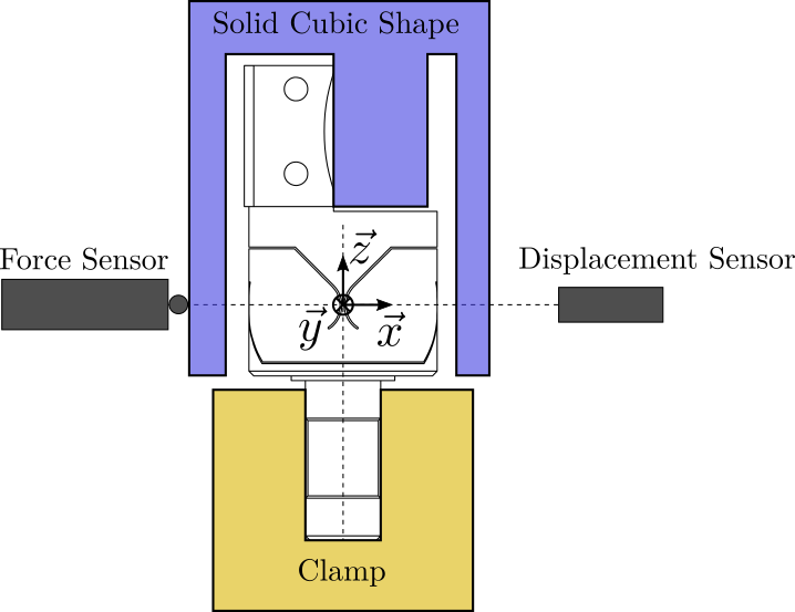
Figure 1: Test bench geometry and axis

3 Shear

3.1 Setup

The applied force as well as the measured displacement are aligned with the flexible joint’s center (Figure 1).

Figure 2: Schematic of the test bench to measure the shear stiffness

Ideally, only shear is induced by the force.

If the force is not exactly aligned with the rotation point of the flexible joint:

in the y-direction: some parasitic torsional motion will be induced
in the z-direction: some parasitic bending motion will be induced

We wish here to estimate how precise the force vector should be aligned with the flexible point in order for the motion measured is mainly due to shear effects and not torsional and bending effects.

3.2 Effect of Shear

The shear effect is simply:

\begin{equation} X_s = \frac{F}{k_s} \end{equation}

3.3 Effect of Bending

If the flexible joint is not perfectly positioned as shown in Figure 3 (offset along the z-axis), the applied force will induce a bending motion in addition to the shear motion.

Figure 3: Considering a position error \(\epsilon_z\) of the measurement and force application point with respect ot the flexible joint center (Side View)

Let’s estimate this effect.

The effect of the vertical position error \(\epsilon_z\) is the apparition of a “bending” torque:

\begin{equation} M_b = \epsilon_z \cdot F \end{equation}

This torque will induce a bending motion \(\theta_y\) of the flexible joint:

\begin{equation} \theta_y = \frac{M_b}{k_b} = \frac{\epsilon_z \cdot F}{k_b} \end{equation}

This rotation will induce an error \(\epsilon_{\theta_y}\) on the measured displacement:

\begin{equation} \epsilon_{\theta_y} = \tan(\theta_y) \epsilon_z - L\left( 1 - \frac{1}{\cos(\theta_y)} \right) \end{equation}

Supposing \(\theta_y\) small:

\begin{equation} \epsilon_{\theta_y} \approx \frac{\epsilon_z^2 \cdot F}{k_b} \left( 1 + \frac{L}{2} \frac{F}{k_b} \right) \end{equation}

And this error to be very small compared to the measured motion due to shear:

\begin{equation} \epsilon_{\theta_y} \ll X_s \end{equation}

Which is equivalent to:

\begin{equation} \epsilon_z \ll \sqrt{\frac{k_b}{k_s} \frac{1}{1 + \frac{L}{2} \frac{F}{k_b}}} \end{equation}

For realistic values, this is almost equivalent to:

\begin{equation} \epsilon_z \ll \sqrt{\frac{k_b}{k_s}} \end{equation}

Numerically:

L = 5e-2; % [m]
F = 20;   % [N]

epsilon_z_max = sqrt(kb/ks/(1 + L/2*F/kb)); % [m]

	10% error	1% error	0.1% error
\(\epsilon_z\,[\mu m]\)	59.1	5.9	0.6

3.4 Effect of Torsion

If the flexible joint is not perfectly positioned as shown in Figure 4 (offset along the y-axis), the applied force will induce a torsional motion in addition to the shear motion.

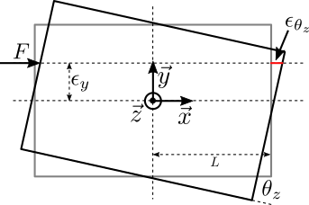
Figure 4: Considering a position error \(\epsilon_y\) of the measurement and force application point with respect ot the flexible joint center (top view)

Let’s estimate this effect.

The effect of the horizontal position error \(\epsilon_y\) is the apparition of a “torsional” torque:

\begin{equation} M_t = \epsilon_y \cdot F \end{equation}

This torque will induce a torsional motion \(\theta_z\) of the flexible joint:

\begin{equation} \theta_z = \frac{M_t}{k_t} = \frac{\epsilon_y \cdot F}{k_t} \end{equation}

This rotation will induce an error \(\epsilon_{\theta_z}\) on the measured displacement:

\begin{equation} \epsilon_{\theta_z} = \tan(\theta_z) \epsilon_y - L\left( 1 - \frac{1}{\cos(\theta_z)} \right) \end{equation}

Supposing \(\theta_z\) small:

\begin{equation} \epsilon_{\theta_z} \approx \frac{\epsilon_y^2 \cdot F}{k_t} \left( 1 + \frac{L}{2} \frac{F}{k_t} \right) \end{equation}

We want this error to be very small compared to the measured motion due to shear:

\begin{equation} \epsilon_{\theta_z} \ll X_s \end{equation}

Which is equivalent to:

\begin{equation} \epsilon_y \ll \sqrt{\frac{k_t}{k_s} \frac{1}{1 + \frac{L}{2} \frac{F}{k_t}}} \end{equation}

For realistic values, this is almost equivalent to:

\begin{equation} \epsilon_y \ll \sqrt{\frac{k_t}{k_s}} \end{equation}

Numerically:

L = 5e-2; % [m]
F = 20;   % [N]

epsilon_y_max = sqrt(kt/ks/(1 + L/2*F/kt)); % [m]

	10% error	1% error	0.1% error
\(\epsilon_y\,[\mu m]\)	446.8	44.7	4.5

4 Axial

4.1 Setup

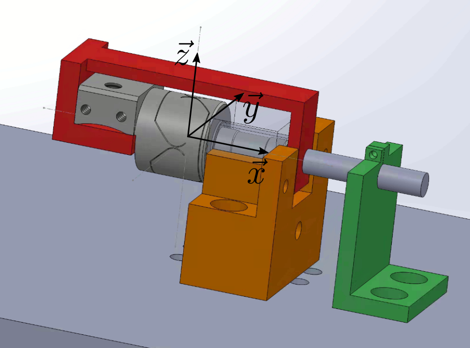
Figure 5: Schematic of the test bench to measure the Axial Stiffness

4.2 Effect of Compression

The axial (compression) effect is simply:

\begin{equation} X_a = \frac{F}{k_a} \end{equation}

4.3 Effect of Bending

If the force is not exactly aligned with the rotation point of the flexible joint, some parasitic bending motion will be induced (Figure 6).

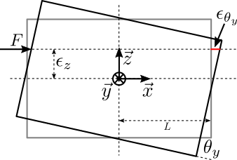
Figure 6: Error of position of the force vector and measurement point with respect to the flexible joint’s center

We wish here to estimate how close to the rotation point the force vector should be aligned for the motion measured to be mainly due to shear effects and not bending effects.

Suppose there is a distance \(\epsilon_z\) form the center of rotation, it will induce a torque equal to:

\begin{equation} M_b = \epsilon_z \cdot F \end{equation}

Therefore, the rotation of the top part will be:

\begin{equation} X_b = \frac{M_b}{k_b} = \frac{\epsilon_z \cdot F}{k_b} \end{equation}

And the induced measured displacement is:

\begin{equation} D_b = \tan(X_b) \epsilon_z - L\left( 1 - \frac{1}{\cos(X_b)} \right) \\ \end{equation}

Supposing \(X_b\) small:

\begin{equation} D_b \approx \frac{\epsilon_z^2 \cdot F}{k_b} \left( 1 + \frac{L}{2} \frac{F}{k_b} \right) \end{equation}

We want the induced displacement due to the bending much smaller than the induced displacement due to the compression:

\begin{equation} D_b \ll Xs \end{equation}

Which is equivalent to (taking \(\tan x \approx x\)):

\begin{equation} \epsilon_z \ll \sqrt{\frac{k_b}{k_a} \frac{1}{1 + \frac{L}{2} \frac{F}{k_b}}} \end{equation}

For realistic values, this is almost equivalent to:

\begin{equation} \epsilon_z \ll \sqrt{\frac{k_b}{k_a}} \end{equation}

Note that an error in \(z\) is chosen here, but the same results are obtained for errors in the \(y\) direction. What matters is the distance from the axis \(F\) to the flexible joint’s center.

Numerically:

L = 10e-2; % [m]
F = 50; % [N]
d_off_eq = sqrt(kb/ka/(1 + L/2*F/kb))

	10% error	1% error	0.1% error
\(\epsilon_y\,[\mu m]\)	18.8	1.9	0.2
\(\epsilon_z\,[\mu m]\)	18.8	1.9	0.2

Same as for the shear measurement, it is very difficult to be that precise, and therefore rotations should also be measured and compensated for.

4.4 Measured Displacement with realistic positioning errors

Suppose there is a positioning error of \(\epsilon_z = 0.1\,mm\).

\begin{equation} X_b = \frac{\epsilon_z \cdot F}{k_b} \end{equation}

Fmax = Fa;
Ez = 0.1e-3;
Xb_max = Ez*Fmax/kb;

Xbmax = 9.4 [mrad]

Which is about half of the maximum stroke in bending.

The

\begin{equation} D_b = \tan(X_b) \epsilon_z - L\left( 1 - \frac{1}{\cos(X_b)} \right) \\ \end{equation}

5 Bending Stiffness

5.1 Setup

Let’s say a force is applied on top of the flexible joint with a distance \(H\) with the joint’s center.

The displacement of the flexible joint is also measure at the same height \(H\).

5.2 Effect of Bending

The torque applied is:

\begin{equation} M_b = F \cdot H \end{equation}

The flexible joint is experiencing a rotation \(R_b\) due to the torque \(M_b\):

\begin{equation} R_b = \frac{M_b}{k_b} = \frac{F \cdot H}{k_b} \end{equation}

This rotation is then measured by the displacement sensor coaxial with the force actuator. The measured displacement is:

\begin{equation} D_b \approx H \tan (R_b) \approx \frac{F \cdot H^2}{k_b} \end{equation}

5.3 Effect of Shear

The effect of Shear on the measured displacement is simply:

\begin{equation} D_s = \frac{F}{k_s} \end{equation}

We would like to have this displacement much smaller than the displacement induced by the bending effects:

\begin{equation} D_b \gg D_s \end{equation}

Which is equivalent as to have:

\begin{equation} H \gg \sqrt{\frac{k_b}{k_s}} \end{equation}

	10% error	1% error	0.1% error
D offset [mm]	6	62	620

We should therefore apply a force at least 50mm higher than the joint’s center for the shear effects to be negligible.

5.4 Effect of Torsion

If the application force is not aligned with the vertical axis of the flexible joint, this will induce a torsion motion that will induce a measurement error.

Let’s note the offset \(x_{off}\):

\begin{equation} D_t \approx \frac{x_{off}^2 \cdot F}{k_t} \left( 1 + \frac{L}{2} \frac{F}{k_t} \right) \end{equation}

And we would like to have:

\begin{equation} D_b \gg D_t \end{equation}

Which is equivalent as to have:

\begin{equation} x_{off} \ll H \sqrt{\frac{k_t}{k_b}} \end{equation}

Let’s take \(H = 50/,mm\).

	10% error	1% error	0.1% error
X offset [mm]	36.1	3.6	0.4

The effect of torsion should be negligible for a positioning accuracy of ~1mm.

5.5 Full stroke measured displacement and applied force as a function of \(H\)

Applying a force with a large offset \(H\) means the induced rotation (for constant force) will be larger. This also means that the measured displacement \(D_b\) will also be larger.

\begin{equation} D_b \approx H \tan (R_b) \end{equation}

Note that we here suppose the force axis is co-linear with the measurement axis.

Let’s compute:

\(D_b\) as a function of \(H\) \[ D_b \approx H \tan (R_b) \]
the applied force \(F_{\text{max}}\) to induce the maximum rotation \[ F_{\text{max}} \approx \frac{X_b \cdot k_b}{H} \]

H = linspace(0, 100e-3, 1000);

Db = H*tan(Xb);
Fmax = Xb*kb./H;

figure;
yyaxis left
plot(1e3*H, Fmax);
ylabel('Maximum Force [$N$]');
ylim([0, 100]);

yyaxis right
plot(1e3*H, 1e6*Db);
ylabel('Measurement Range [$\mu m$]');

xlabel('Offset $H$ [$mm$]');

5.6 Conclusion

Applied Force
Measured Displacement
Requirements in terms of positioning

6 Torsion

6.1 Distance to flex axis for torsion >> shear

6.2 Force Location Precision for torsion >> bending

7 Force Sensor

Requirements:

Large enough measurement range
Small enough measurement noise and errors

The largest applied force is foreseen to be around 500N. The smallest (full range) force is foreseen to be around 2N.

If we want an accuracy of 1% (even for the small measurement range), the force sensor should be accurate down to ~0.02N and with a full range of 500N. This corresponds to an accuracy of 0.004%.

If we limit ourselves to 100N of applied force, the required accuracy of 0.02N corresponds to 0.02% of accuracy which is more realistic.

Another solution would be to use 2 force sensors.

Fmax = 500; % [N]
Fmin = 2; % [N]
Fres = Fmin/100; % [N]

% Dynamic range
Fmax/Fres

Model	Range [N]	Accuracy	Error [N]
S2M	100	0.02%	0.02
S2M	500	0.02%	0.1
ALF241	100	0.05%	0.05
PM1500	500	0.05%	0.5

https://www.hbm.com/en/2925/top-transfer-reference-force-transducer-maximum-precision/

State of the art but big

https://www.burster.com//en/sensors/load-cells/high-precision-load-cells/p/detail/8527

500N range => 0.25N error

8 Displacement Sensor

8.1 Three displacement sensors to measure both rotations \(\theta_y,\theta_z\) and translation \(x\)

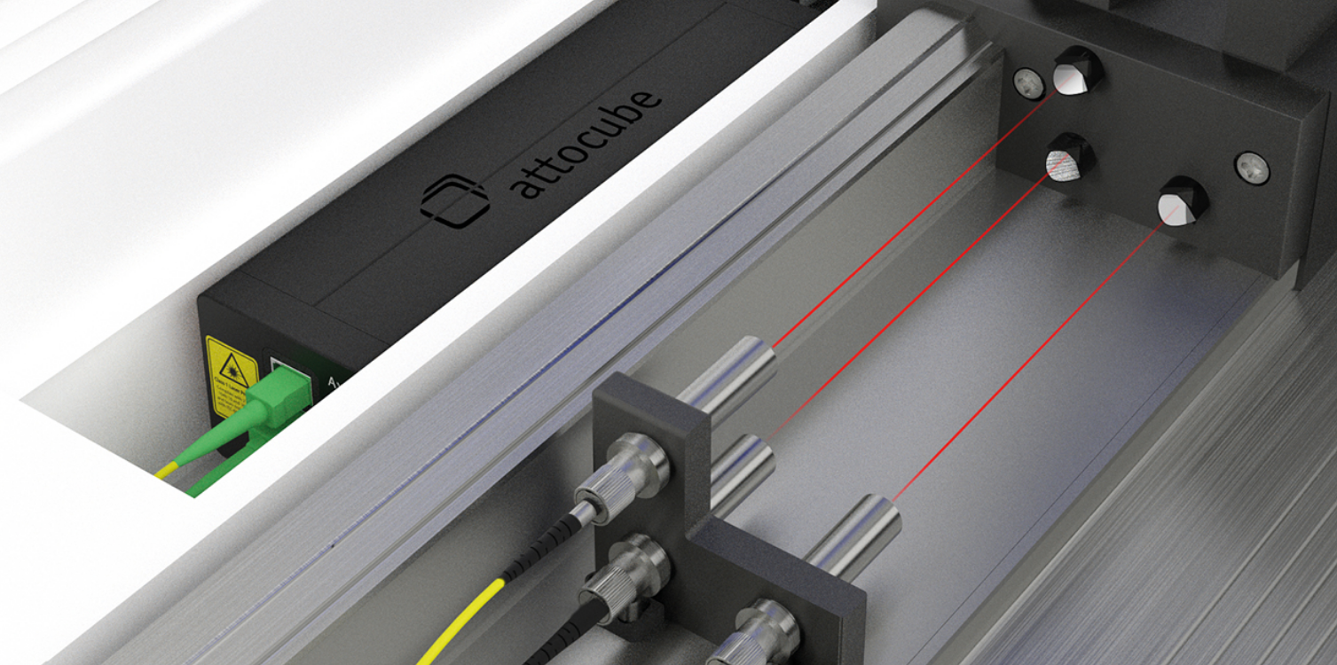
Figure 7: Figure caption

Capacitive sensors or interferometers
Choice of the position of the three sensors => will change rotation sensitivity and range

Flexible Joint - Test Bench

Table of Contents

1 Finite Element Model

1.1 Parameters

2 Measurement Setup

3 Shear

3.1 Setup

3.2 Effect of Shear

3.3 Effect of Bending

3.4 Effect of Torsion

4 Axial

4.1 Setup

4.2 Effect of Compression

4.3 Effect of Bending

4.4 Measured Displacement with realistic positioning errors

5 Bending Stiffness

5.1 Setup

5.2 Effect of Bending

5.3 Effect of Shear

5.4 Effect of Torsion

5.5 Full stroke measured displacement and applied force as a function of \(H\)

5.6 Conclusion

6 Torsion

6.1 Distance to flex axis for torsion >> shear

6.2 Force Location Precision for torsion >> bending

7 Force Sensor

8 Displacement Sensor

8.1 Three displacement sensors to measure both rotations \(\theta_y,\theta_z\) and translation \(x\)