Amplifier Piezoelectric Actuator APA300ML - Test Bench
Table of Contents
- 1. Model of an Amplified Piezoelectric Actuator and Sensor
- 2. Geometrical Measurements
- 3. Electrical Measurements
- 4. Stiffness measurement
- 5. Stroke measurement
- 6. Test-Bench Description
- 7. Measurement Procedure
- 8. Measurement Results
- 9. Test Bench APA300ML - Simscape Model
- 10. Test Bench Struts - Simscape Model
- 11. Resonance frequencies - APA300ML
This report is also available as a pdf.
The goal of this test bench is to extract all the important parameters of the Amplified Piezoelectric Actuator APA300ML.
This include:
- Stroke
- Stiffness
- Hysteresis
- Gain from the applied voltage \(V_a\) to the generated Force \(F_a\)
- Gain from the sensor stack strain \(\delta L\) to the generated voltage \(V_s\)
- Dynamical behavior
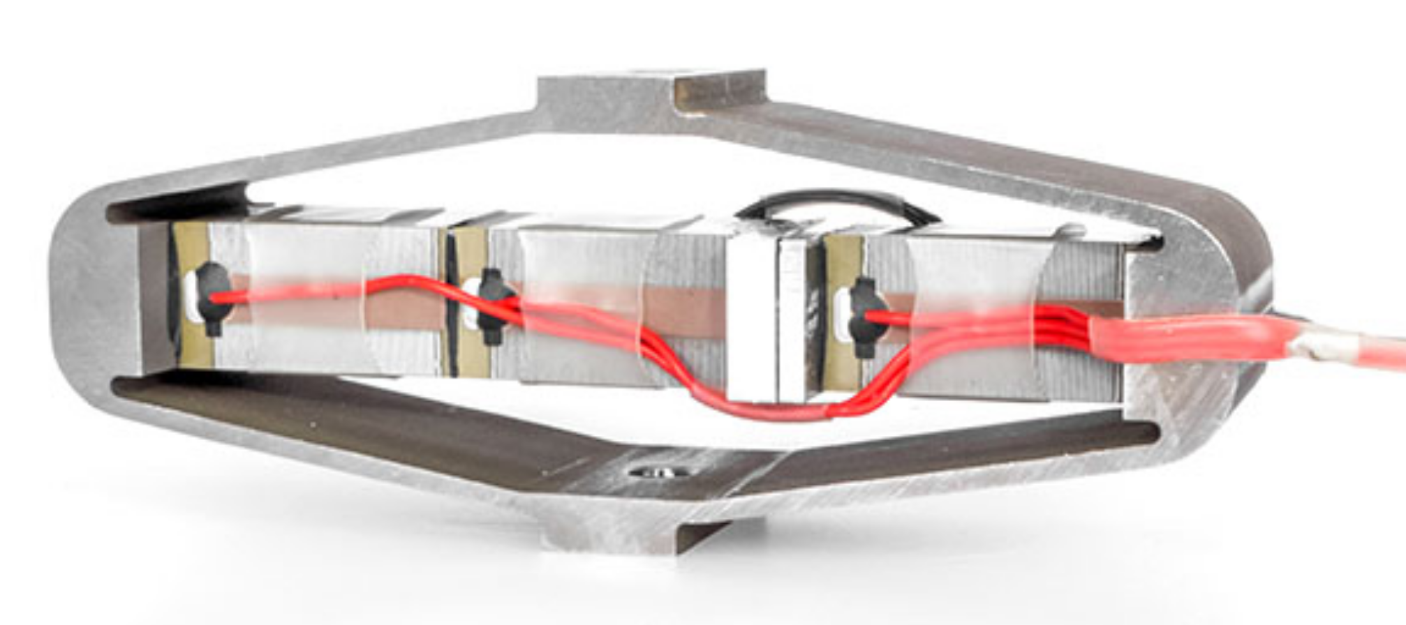
Figure 1: Picture of the APA300ML
1 Model of an Amplified Piezoelectric Actuator and Sensor
Consider a schematic of the Amplified Piezoelectric Actuator in Figure 2.
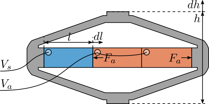
Figure 2: Amplified Piezoelectric Actuator Schematic
A voltage \(V_a\) applied to the actuator stacks will induce an actuator force \(F_a\):
\begin{equation} F_a = g_a \cdot V_a \end{equation}A change of length \(dl\) of the sensor stack will induce a voltage \(V_s\):
\begin{equation} V_s = g_s \cdot dl \end{equation}We wish here to experimental measure \(g_a\) and \(g_s\).
The block-diagram model of the piezoelectric actuator is then as shown in Figure 3.

Figure 3: Model of the APA with Simscape/Simulink
2 Geometrical Measurements
The received APA are shown in Figure 4.
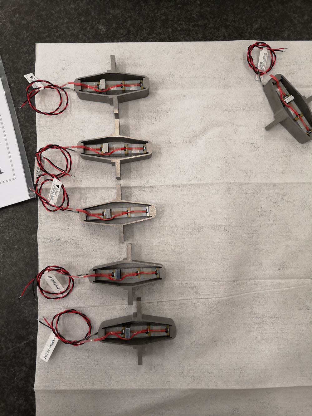
Figure 4: Received APA
2.1 Measurement Setup
The flatness corresponding to the two interface planes are measured as shown in Figure 5.
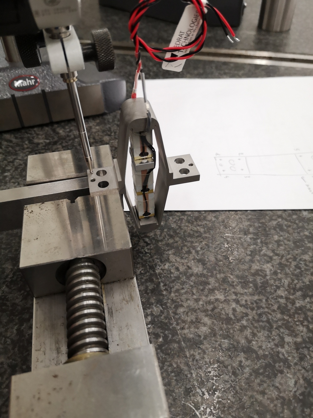
Figure 5: Measurement Setup
2.2 Measurement Results
The height (Z) measurements at the 8 locations (4 points by plane) are defined below.
apa1  = 1e-6*[0, -0.5 , 3.5  , 3.5  , 42   , 45.5, 52.5 , 46];
apa2  = 1e-6*[0, -2.5 , -3   , 0    , -1.5 , 1   , -2   , -4];
apa3  = 1e-6*[0, -1.5 , 15   , 17.5 , 6.5  , 6.5 , 21   , 23];
apa4  = 1e-6*[0, 6.5  , 14.5 , 9    , 16   , 22  , 29.5 , 21];
apa5  = 1e-6*[0, -12.5, 16.5 , 28.5 , -43  , -52 , -22.5, -13.5];
apa6  = 1e-6*[0, -8   , -2   , 5    , -57.5, -62 , -55.5, -52.5];
apa7  = 1e-6*[0, 19.5 , -8   , -29.5, 75   , 97.5, 70   , 48];
apa7b = 1e-6*[0, 9    , -18.5, -30  , 31   , 46.5, 16.5 , 7.5];
apa = {apa1, apa2, apa3, apa4, apa5, apa6, apa7b};
The X/Y Positions of the 8 measurement points are defined below.
W = 20e-3;   % Width [m]
L = 61e-3;   % Length [m]
d = 1e-3;    % Distance from border [m]
l = 15.5e-3; % [m]

pos = [[-L/2 + d; W/2 - d], [-L/2 + l - d; W/2 - d], [-L/2 + l - d; -W/2 + d], [-L/2 + d; -W/2 + d], [L/2 - l + d; W/2 - d], [L/2 - d; W/2 - d], [L/2 - d; -W/2 + d], [L/2 - l + d; -W/2 + d]];
Finally, the flatness is estimated by fitting a plane through the 8 points using the fminsearch command.
apa_d = zeros(1, 7);
for i = 1:7
    fun = @(x)max(abs(([pos; apa{i}]-[0;0;x(1)])'*([x(2:3);1]/norm([x(2:3);1]))));
    x0 = [0;0;0];
    [x, min_d] = fminsearch(fun,x0);
    apa_d(i) = min_d;
end
The obtained flatness are shown in Table 1.
| Flatness \([\mu m]\) | |
|---|---|
| APA 1 | 8.9 |
| APA 2 | 3.1 |
| APA 3 | 9.1 |
| APA 4 | 3.0 |
| APA 5 | 1.9 |
| APA 6 | 7.1 |
| APA 7 | 18.7 |
3 Electrical Measurements
The capacitance of the stacks is measure with the LCR-800 Meter (doc)

Figure 6: LCR Meter used for the measurements
The excitation frequency is set to be 1kHz.
| Sensor Stack | Actuator Stacks | |
|---|---|---|
| APA 1 | 5.10 | 10.03 |
| APA 2 | 4.99 | 9.85 |
| APA 3 | 1.72 | 5.18 |
| APA 4 | 4.94 | 9.82 |
| APA 5 | 4.90 | 9.66 |
| APA 6 | 4.99 | 9.91 |
| APA 7 | 4.85 | 9.85 |
There is clearly a problem with APA300ML number 3
4 Stiffness measurement
4.1 APA test
load('meas_stiff_apa_1_x.mat', 't', 'F', 'd');
figure;
plot(t, F)
%% Automatic Zero of the force
F = F - mean(F(t > 0.1 & t < 0.3));

%% Start measurement at t = 0.2 s
d = d(t > 0.2);
F = F(t > 0.2);
t = t(t > 0.2); t = t - t(1);
i_l_start = find(F > 0.3, 1, 'first');
[~, i_l_stop] = max(F);
F_l = F(i_l_start:i_l_stop);
d_l = d(i_l_start:i_l_stop);
fit_l = polyfit(F_l, d_l, 1);

% %% Reset displacement based on fit
% d = d - fit_l(2);
% fit_s(2) = fit_s(2) - fit_l(2);
% fit_l(2) = 0;

% %% Estimated Stroke
% F_max = fit_s(2)/(fit_l(1) - fit_s(1));
% d_max = fit_l(1)*F_max;
h^2/fit_l(1)
figure;
hold on;
plot(F,d,'k')
plot(F_l, d_l)
plot(F_l, F_l*fit_l(1) + fit_l(2), '--')
5 Stroke measurement
We here wish to estimate the stroke of the APA.
To do so, one side of the APA is fixed, and a displacement probe is located on the other side as shown in Figure 7.
Then, a voltage is applied on either one or two stacks using a DAC and a voltage amplifier.
Here are the documentation of the equipment used for this test bench:
- Voltage Amplifier: PD200 with a gain of 20
- 16bits DAC: IO313 Speedgoat card
- Displacement Probe: Millimar C1216 electronics and Millimar 1318 probe

Figure 7: Bench to measured the APA stroke
5.1 Voltage applied on one stack
Let’s first look at the relation between the voltage applied to one stack to the displacement of the APA as measured by the displacement probe.
The applied voltage is shown in Figure 8.
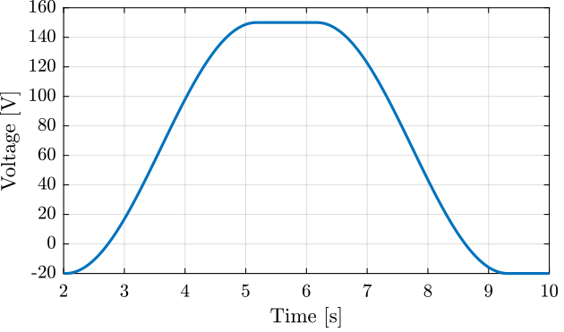
Figure 8: Applied voltage as a function of time
The obtained displacement is shown in Figure 9. The displacement is set to zero at initial time when the voltage applied is -20V.
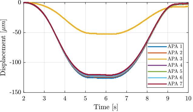
Figure 9: Displacement as a function of time for all the APA300ML
Finally, the displacement is shown as a function of the applied voltage in Figure 10. We can clearly see that there is a problem with the APA 3. Also, there is a large hysteresis.

Figure 10: Displacement as a function of the applied voltage
We can clearly see from Figure 10 that there is a problem with the APA number 3.
5.2 Voltage applied on two stacks
Now look at the relation between the voltage applied to the two other stacks to the displacement of the APA as measured by the displacement probe.
The obtained displacement is shown in Figure 11. The displacement is set to zero at initial time when the voltage applied is -20V.
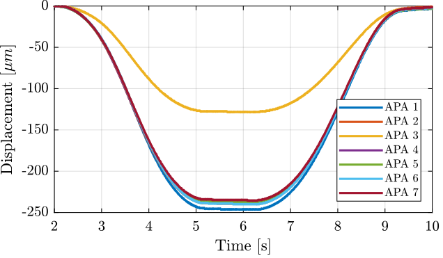
Figure 11: Displacement as a function of time for all the APA300ML
Finally, the displacement is shown as a function of the applied voltage in Figure 12. We can clearly see that there is a problem with the APA 3. Also, there is a large hysteresis.

Figure 12: Displacement as a function of the applied voltage
5.3 Voltage applied on all three stacks
Finally, we can combine the two measurements to estimate the relation between the displacement and the voltage applied to the three stacks (Figure 13).
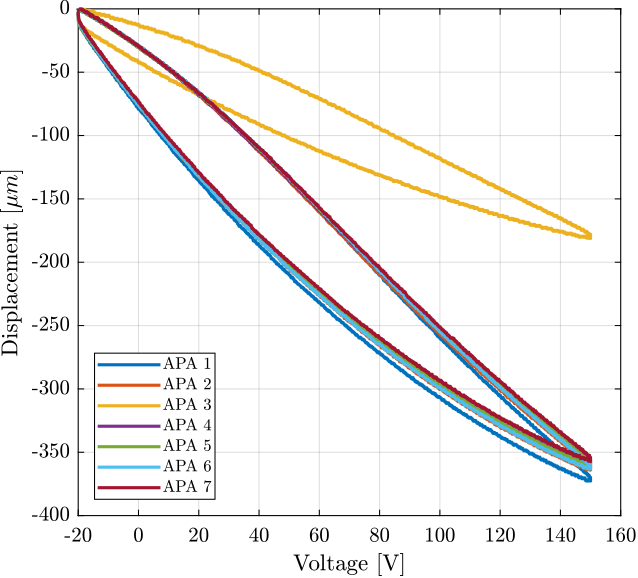
Figure 13: Displacement as a function of the applied voltage
The obtained maximum stroke for all the APA are summarized in Table 3.
| Stroke \([\mu m]\) | |
|---|---|
| APA 1 | 373.2 |
| APA 2 | 365.5 |
| APA 3 | 181.7 |
| APA 4 | 359.7 |
| APA 5 | 361.5 |
| APA 6 | 363.9 |
| APA 7 | 358.4 |
6 Test-Bench Description
Here are the documentation of the equipment used for this test bench:
- Voltage Amplifier: PD200
- Amplified Piezoelectric Actuator: APA300ML
- DAC/ADC: Speedgoat IO313
- Encoder: Renishaw Vionic and used Ruler
- Interferometer: Attocube IDS3010

Figure 14: Schematic of the Test Bench
7 Measurement Procedure
7.1 Stroke Measurement
Using the PD200 amplifier, output a voltage: \[ V_a = 65 + 85 \sin(2\pi \cdot t) \] To have a quasi-static excitation between -20 and 150V.
As the gain of the PD200 amplifier is 20, the DAC output voltage should be: \[ V_{dac}(t) = 3.25 + 4.25\sin(2\pi \cdot t) \]
Verify that the voltage offset of the PD200 is zero!
Measure the output vertical displacement \(d\) using the interferometer.
Then, plot \(d\) as a function of \(V_a\), and perform a linear regression. Conclude on the obtained stroke.
7.2 Stiffness Measurement
Add some (known) weight \(\delta m g\) on the suspended mass and measure the deflection \(\delta d\). This can be tested when the piezoelectric stacks are open-circuit.
As the stiffness will be around \(k \approx 10^6 N/m\), an added mass of \(m \approx 100g\) will induce a static deflection of \(\approx 1\mu m\) which should be large enough for a precise measurement using the interferometer.
Then the obtained stiffness is:
\begin{equation} k = \frac{\delta m g}{\delta d} \end{equation}7.3 Hysteresis measurement
Supply a quasi static sinusoidal excitation \(V_a\) at different voltages.
The offset should be 65V, and the sin amplitude can range from 1V up to 85V.
For each excitation amplitude, the vertical displacement \(d\) of the mass is measured.
Then, \(d\) is plotted as a function of \(V_a\) for all the amplitudes.

Figure 15: Expected Hysteresis (poel10_explor_activ_hard_mount_vibrat)
7.4 Piezoelectric Actuator Constant
Using the measurement test-bench, it is rather easy the determine the static gain between the applied voltage \(V_a\) to the induced displacement \(d\). Use a quasi static (1Hz) excitation signal \(V_a\) on the piezoelectric stack and measure the vertical displacement \(d\). Perform a linear regression to obtain:
\begin{equation} d = g_{d/V_a} \cdot V_a \end{equation}Using the Simscape model of the APA, it is possible to determine the static gain between the actuator force \(F_a\) to the induced displacement \(d\):
\begin{equation} d = g_{d/F_a} \cdot F_a \end{equation}From the two gains, it is then easy to determine \(g_a\):
\begin{equation} g_a = \frac{F_a}{V_a} = \frac{F_a}{d} \cdot \frac{d}{V_a} = \frac{g_{d/V_a}}{g_{d/F_a}} \end{equation}7.5 Piezoelectric Sensor Constant
From a quasi static excitation of the piezoelectric stack, measure the gain from \(V_a\) to \(V_s\):
\begin{equation} V_s = g_{V_s/V_a} V_a \end{equation}Note here that there is an high pass filter formed by the piezo capacitor and parallel resistor. The excitation frequency should then be in between the cut-off frequency of this high pass filter and the first resonance.
Alternatively, the gain can be computed from the dynamical identification and taking the gain at the wanted frequency.
Using the simscape model, compute the static gain from the actuator force \(F_a\) to the strain of the sensor stack \(dl\):
\begin{equation} dl = g_{dl/F_a} F_a \end{equation}Then, the static gain from the sensor stack strain \(dl\) to the general voltage \(V_s\) is:
\begin{equation} g_s = \frac{V_s}{dl} = \frac{V_s}{V_a} \cdot \frac{V_a}{F_a} \cdot \frac{F_a}{dl} = \frac{g_{V_s/V_a}}{g_a \cdot g_{dl/F_a}} \end{equation}Alternatively, we could impose an external force to add strain in the APA that should be equally present in all the 3 stacks and equal to 1/5 of the vertical strain. This external force can be some weight added, or a piezo in parallel.
7.6 Capacitance Measurement
Measure the capacitance of the 3 stacks individually using a precise multi-meter.
7.7 Dynamical Behavior
Perform a system identification from \(V_a\) to the measured displacement \(d\) by the interferometer and by the encoder, and to the generated voltage \(V_s\).
This can be performed using different excitation signals.
This can also be performed with and without the encoder fixed to the APA.
7.8 Compare the results obtained for all 7 APA300ML
Compare all the obtained parameters for all the test APA.
8 Measurement Results
9 Test Bench APA300ML - Simscape Model
9.1 Introduction
9.2 Nano Hexapod object
n_hexapod = struct();
9.2.1 APA - 2 DoF
n_hexapod.actuator = struct();

n_hexapod.actuator.type = 1;

n_hexapod.actuator.k  = ones(6,1)*0.35e6; % [N/m]
n_hexapod.actuator.ke = ones(6,1)*1.5e6; % [N/m]
n_hexapod.actuator.ka = ones(6,1)*43e6; % [N/m]

n_hexapod.actuator.c  = ones(6,1)*3e1; % [N/(m/s)]
n_hexapod.actuator.ce = ones(6,1)*1e1; % [N/(m/s)]
n_hexapod.actuator.ca = ones(6,1)*1e1; % [N/(m/s)]

n_hexapod.actuator.Leq = ones(6,1)*0.056; % [m]

n_hexapod.actuator.Ga = ones(6,1)*1; % Actuator gain [N/V]
n_hexapod.actuator.Gs = ones(6,1)*1; % Sensor gain [V/m]
9.2.2 APA - Flexible Frame
n_hexapod.actuator.type = 2;

n_hexapod.actuator.K = readmatrix('APA300ML_b_mat_K.CSV'); % Stiffness Matrix
n_hexapod.actuator.M = readmatrix('APA300ML_b_mat_M.CSV'); % Mass Matrix
n_hexapod.actuator.xi = 0.01; % Damping ratio
n_hexapod.actuator.P = extractNodes('APA300ML_b_out_nodes_3D.txt'); % Node coordinates [m]

n_hexapod.actuator.ks = 235e6; % Stiffness of one stack [N/m]
n_hexapod.actuator.cs = 1e1; % Stiffness of one stack [N/m]

n_hexapod.actuator.Ga = ones(6,1)*1; % Actuator gain [N/V]
n_hexapod.actuator.Gs = ones(6,1)*1; % Sensor gain [V/m]
9.2.3 APA - Fully Flexible
n_hexapod.actuator.type = 3;

n_hexapod.actuator.K = readmatrix('APA300ML_full_mat_K.CSV'); % Stiffness Matrix
n_hexapod.actuator.M = readmatrix('APA300ML_full_mat_M.CSV'); % Mass Matrix
n_hexapod.actuator.xi = 0.01; % Damping ratio
n_hexapod.actuator.P = extractNodes('APA300ML_full_out_nodes_3D.txt'); % Node coordiantes [m]

n_hexapod.actuator.Ga = ones(6,1)*1; % Actuator gain [N/V]
n_hexapod.actuator.Gs = ones(6,1)*1; % Sensor gain [V/m]
9.3 Identification
%% Options for Linearized
options = linearizeOptions;
options.SampleTime = 0;

%% Name of the Simulink File
mdl = 'test_bench_apa300ml';

%% Input/Output definition
clear io; io_i = 1;
io(io_i) = linio([mdl, '/Va'],  1, 'openinput');  io_i = io_i + 1; % Actuator Voltage
io(io_i) = linio([mdl, '/Vs'],  1, 'openoutput'); io_i = io_i + 1; % Sensor Voltage
io(io_i) = linio([mdl, '/dL'],  1, 'openoutput'); io_i = io_i + 1; % Relative Motion Outputs
io(io_i) = linio([mdl, '/z'],   1, 'openoutput'); io_i = io_i + 1; % Vertical Motion

%% Run the linearization
Ga = linearize(mdl, io, 0.0, options);
Ga.InputName  = {'Va'};
Ga.OutputName = {'Vs', 'dL', 'z'};
9.4 Compare 2-DoF with flexible
9.4.1 APA - 2 DoF
n_hexapod = struct();

n_hexapod.actuator = struct();

n_hexapod.actuator.type = 1;

n_hexapod.actuator.k  = ones(6,1)*0.35e6; % [N/m]
n_hexapod.actuator.ke = ones(6,1)*1.5e6; % [N/m]
n_hexapod.actuator.ka = ones(6,1)*43e6; % [N/m]

n_hexapod.actuator.c  = ones(6,1)*3e1; % [N/(m/s)]
n_hexapod.actuator.ce = ones(6,1)*1e1; % [N/(m/s)]
n_hexapod.actuator.ca = ones(6,1)*1e1; % [N/(m/s)]

n_hexapod.actuator.Leq = ones(6,1)*0.056; % [m]

n_hexapod.actuator.Ga = ones(6,1)*-2.15; % Actuator gain [N/V]
n_hexapod.actuator.Gs = ones(6,1)*2.305e-08; % Sensor gain [V/m]
G_2dof = linearize(mdl, io, 0.0, options);
G_2dof.InputName  = {'Va'};
G_2dof.OutputName = {'Vs', 'dL', 'z'};
9.4.2 APA - Fully Flexible
n_hexapod = struct();

n_hexapod.actuator.type = 3;

n_hexapod.actuator.K = readmatrix('APA300ML_full_mat_K.CSV'); % Stiffness Matrix
n_hexapod.actuator.M = readmatrix('APA300ML_full_mat_M.CSV'); % Mass Matrix
n_hexapod.actuator.xi = 0.01; % Damping ratio
n_hexapod.actuator.P = extractNodes('APA300ML_full_out_nodes_3D.txt'); % Node coordiantes [m]

n_hexapod.actuator.Ga = ones(6,1)*1; % Actuator gain [N/V]
n_hexapod.actuator.Gs = ones(6,1)*1; % Sensor gain [V/m]
G_flex = linearize(mdl, io, 0.0, options);
G_flex.InputName  = {'Va'};
G_flex.OutputName = {'Vs', 'dL', 'z'};
9.4.3 Comparison
10 Test Bench Struts - Simscape Model
10.1 Introduction
10.2 Nano Hexapod object
n_hexapod = struct();
10.2.1 Flexible Joint - Bot
n_hexapod.flex_bot = struct();

n_hexapod.flex_bot.type = 1; % 1: 2dof / 2: 3dof / 3: 4dof

n_hexapod.flex_bot.kRx = ones(6,1)*5; % X bending stiffness [Nm/rad]
n_hexapod.flex_bot.kRy = ones(6,1)*5; % Y bending stiffness [Nm/rad]
n_hexapod.flex_bot.kRz = ones(6,1)*260; % Torsionnal stiffness [Nm/rad]
n_hexapod.flex_bot.kz  = ones(6,1)*1e8; % Axial stiffness [N/m]

n_hexapod.flex_bot.cRx = ones(6,1)*0.1; % [Nm/(rad/s)]
n_hexapod.flex_bot.cRy = ones(6,1)*0.1; % [Nm/(rad/s)]
n_hexapod.flex_bot.cRz = ones(6,1)*0.1; % [Nm/(rad/s)]
n_hexapod.flex_bot.cz  = ones(6,1)*1e2; %[N/(m/s)]
10.2.2 Flexible Joint - Top
n_hexapod.flex_top = struct();

n_hexapod.flex_top.type = 2; % 1: 2dof / 2: 3dof / 3: 4dof

n_hexapod.flex_top.kRx = ones(6,1)*5; % X bending stiffness [Nm/rad]
n_hexapod.flex_top.kRy = ones(6,1)*5; % Y bending stiffness [Nm/rad]
n_hexapod.flex_top.kRz = ones(6,1)*260; % Torsionnal stiffness [Nm/rad]
n_hexapod.flex_top.kz  = ones(6,1)*1e8; % Axial stiffness [N/m]

n_hexapod.flex_top.cRx = ones(6,1)*0.1; % [Nm/(rad/s)]
n_hexapod.flex_top.cRy = ones(6,1)*0.1; % [Nm/(rad/s)]
n_hexapod.flex_top.cRz = ones(6,1)*0.1; % [Nm/(rad/s)]
n_hexapod.flex_top.cz  = ones(6,1)*1e2; %[N/(m/s)]
10.2.3 APA - 2 DoF
n_hexapod.actuator = struct();

n_hexapod.actuator.type = 1;

n_hexapod.actuator.k  = ones(6,1)*0.35e6; % [N/m]
n_hexapod.actuator.ke = ones(6,1)*1.5e6; % [N/m]
n_hexapod.actuator.ka = ones(6,1)*43e6; % [N/m]

n_hexapod.actuator.c  = ones(6,1)*3e1; % [N/(m/s)]
n_hexapod.actuator.ce = ones(6,1)*1e1; % [N/(m/s)]
n_hexapod.actuator.ca = ones(6,1)*1e1; % [N/(m/s)]

n_hexapod.actuator.Leq = ones(6,1)*0.056; % [m]

n_hexapod.actuator.Ga = ones(6,1)*1; % Actuator gain [N/V]
n_hexapod.actuator.Gs = ones(6,1)*1; % Sensor gain [V/m]
10.2.4 APA - Flexible Frame
n_hexapod.actuator.type = 2;

n_hexapod.actuator.K = readmatrix('APA300ML_b_mat_K.CSV'); % Stiffness Matrix
n_hexapod.actuator.M = readmatrix('APA300ML_b_mat_M.CSV'); % Mass Matrix
n_hexapod.actuator.xi = 0.01; % Damping ratio
n_hexapod.actuator.P = extractNodes('APA300ML_b_out_nodes_3D.txt'); % Node coordinates [m]

n_hexapod.actuator.ks = 235e6; % Stiffness of one stack [N/m]
n_hexapod.actuator.cs = 1e1; % Stiffness of one stack [N/m]

n_hexapod.actuator.Ga = ones(6,1)*1; % Actuator gain [N/V]
n_hexapod.actuator.Gs = ones(6,1)*1; % Sensor gain [V/m]
10.2.5 APA - Fully Flexible
n_hexapod.actuator.type = 3;

n_hexapod.actuator.K = readmatrix('APA300ML_full_mat_K.CSV'); % Stiffness Matrix
n_hexapod.actuator.M = readmatrix('APA300ML_full_mat_M.CSV'); % Mass Matrix
n_hexapod.actuator.xi = 0.01; % Damping ratio
n_hexapod.actuator.P = extractNodes('APA300ML_full_out_nodes_3D.txt'); % Node coordiantes [m]

n_hexapod.actuator.Ga = ones(6,1)*1; % Actuator gain [N/V]
n_hexapod.actuator.Gs = ones(6,1)*1; % Sensor gain [V/m]
10.3 Identification
%% Options for Linearized
options = linearizeOptions;
options.SampleTime = 0;

%% Name of the Simulink File
mdl = 'test_bench_struts';

%% Input/Output definition
clear io; io_i = 1;
io(io_i) = linio([mdl, '/Va'],  1, 'openinput');  io_i = io_i + 1; % Actuator Voltage
io(io_i) = linio([mdl, '/Vs'],  1, 'openoutput'); io_i = io_i + 1; % Sensor Voltage
io(io_i) = linio([mdl, '/dL'],  1, 'openoutput'); io_i = io_i + 1; % Relative Motion Outputs
io(io_i) = linio([mdl, '/z'],   1, 'openoutput'); io_i = io_i + 1; % Vertical Motion

%% Run the linearization
Gs = linearize(mdl, io, 0.0, options);
Gs.InputName  = {'Va'};
Gs.OutputName = {'Vs', 'dL', 'z'};
10.4 Compare flexible joints
10.4.1 Perfect
n_hexapod.flex_bot.type = 1; % 1: 2dof / 2: 3dof / 3: 4dof
n_hexapod.flex_top.type = 2; % 1: 2dof / 2: 3dof / 3: 4dof
Gp = linearize(mdl, io, 0.0, options);
Gp.InputName  = {'Va'};
Gp.OutputName = {'Vs', 'dL', 'z'};
10.4.2 Top Flexible
n_hexapod.flex_bot.type = 1; % 1: 2dof / 2: 3dof / 3: 4dof
n_hexapod.flex_top.type = 3; % 1: 2dof / 2: 3dof / 3: 4dof
Gt = linearize(mdl, io, 0.0, options);
Gt.InputName  = {'Va'};
Gt.OutputName = {'Vs', 'dL', 'z'};
10.4.3 Bottom Flexible
n_hexapod.flex_bot.type = 3; % 1: 2dof / 2: 3dof / 3: 4dof
n_hexapod.flex_top.type = 2; % 1: 2dof / 2: 3dof / 3: 4dof
Gb = linearize(mdl, io, 0.0, options);
Gb.InputName  = {'Va'};
Gb.OutputName = {'Vs', 'dL', 'z'};
10.4.4 Both Flexible
n_hexapod.flex_bot.type = 3; % 1: 2dof / 2: 3dof / 3: 4dof
n_hexapod.flex_top.type = 3; % 1: 2dof / 2: 3dof / 3: 4dof
Gf = linearize(mdl, io, 0.0, options);
Gf.InputName  = {'Va'};
Gf.OutputName = {'Vs', 'dL', 'z'};
10.4.5 Comparison
11 Resonance frequencies - APA300ML
11.1 Introduction
Three main resonances are foreseen to be problematic for the control of the APA300ML:
- Mode in X-bending at 189Hz (Figure 16)
- Mode in Y-bending at 285Hz (Figure 17)
- Mode in Z-torsion at 400Hz (Figure 18)
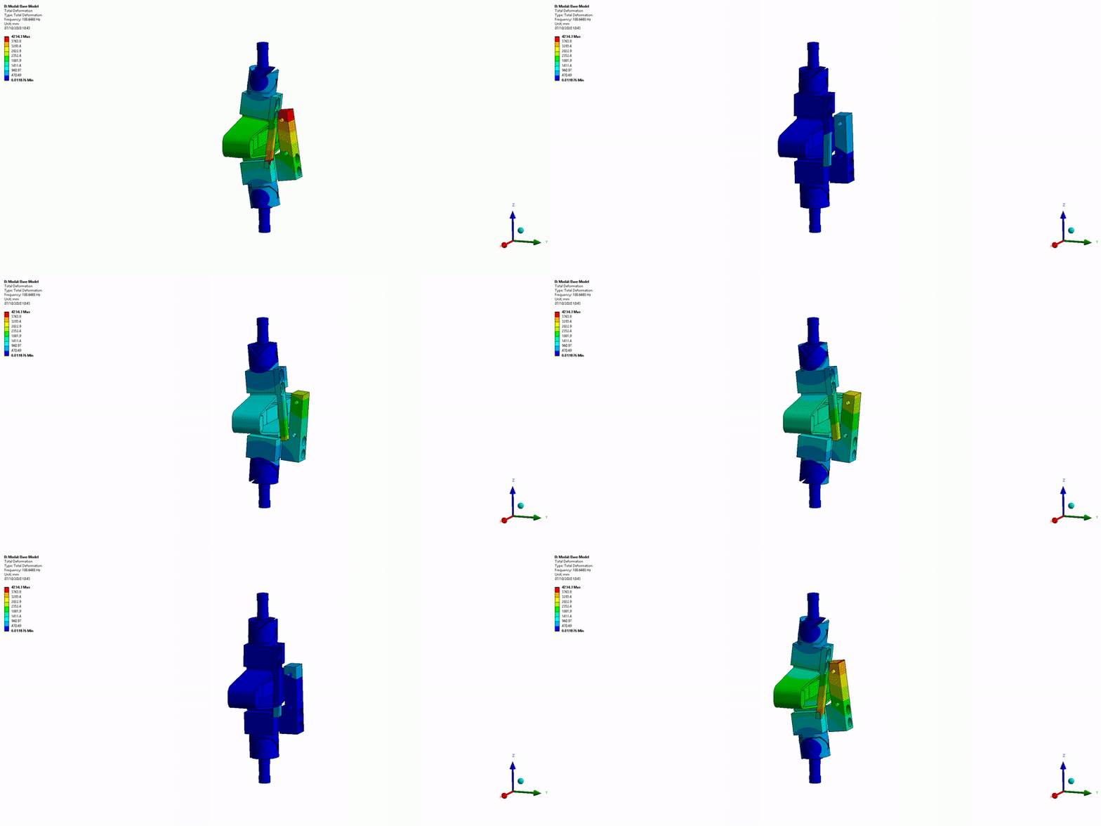
Figure 16: X-bending mode (189Hz)
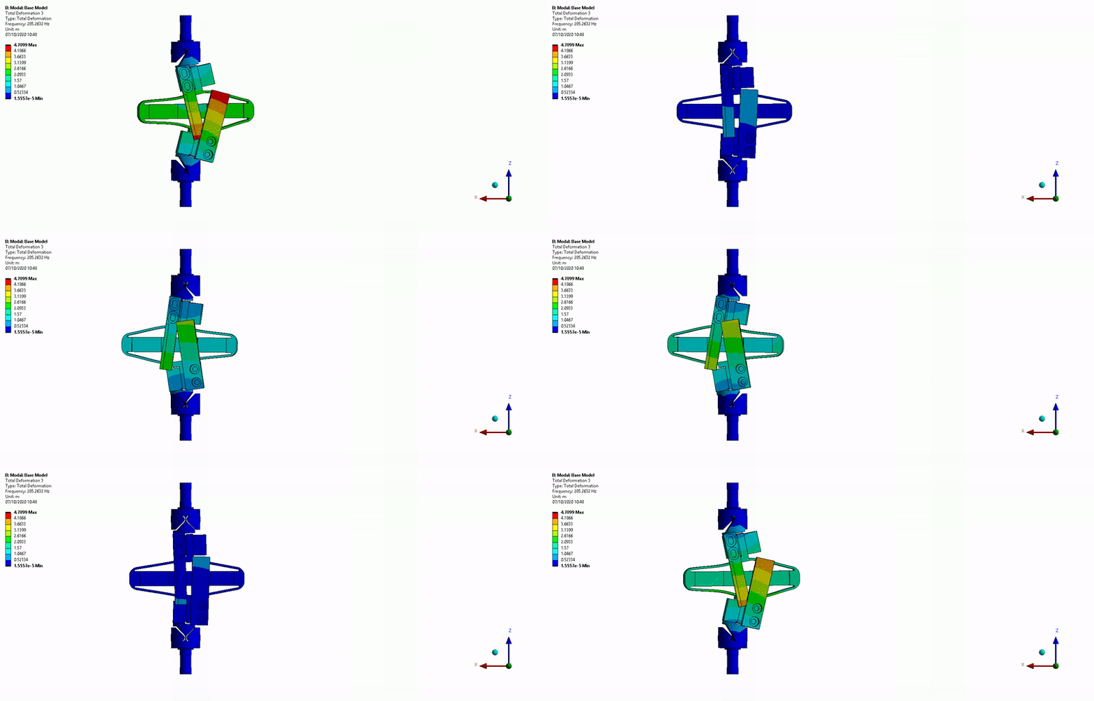
Figure 17: Y-bending mode (285Hz)
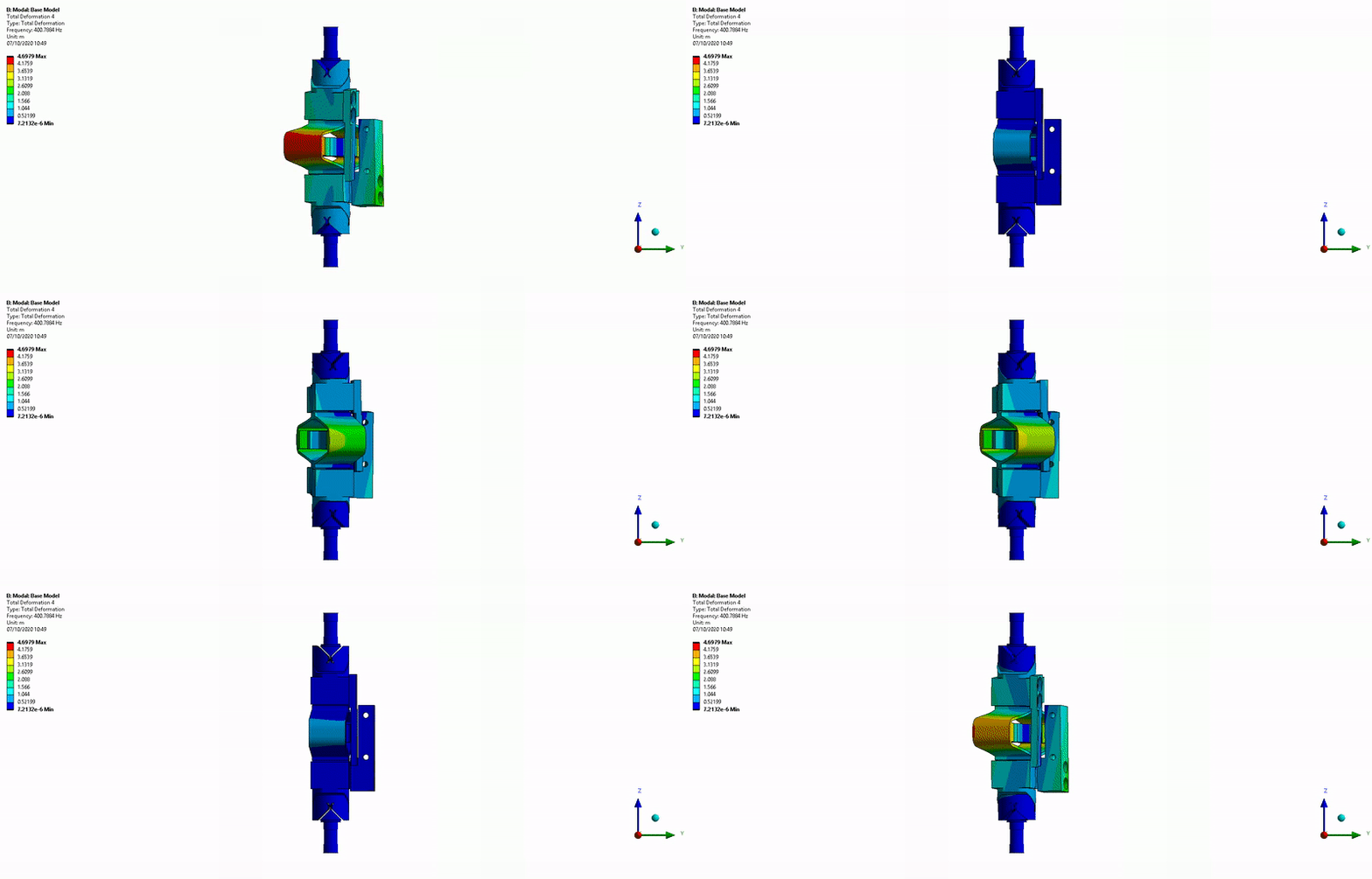
Figure 18: Z-torsion mode (400Hz)
These modes are present when flexible joints are fixed to the ends of the APA300ML.
In this section, we try to find the resonance frequency of these modes when one end of the APA is fixed and the other is free.
11.2 Setup
The measurement setup is shown in Figure 19. A Laser vibrometer is measuring the difference of motion of two points. The APA is excited with an instrumented hammer and the transfer function from the hammer to the measured rotation is computed.
- Laser Doppler Vibrometer Polytec OFV512
- Instrumented hammer
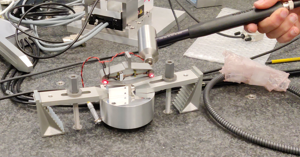
Figure 19: Measurement setup with a Laser Doppler Vibrometer and one instrumental hammer
11.3 Bending - X
The setup to measure the X-bending motion is shown in Figure 20. The APA is excited with an instrumented hammer having a solid metallic tip. The impact point is on the back-side of the APA aligned with the top measurement point.
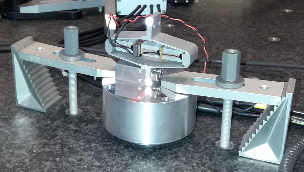
Figure 20: X-Bending measurement setup
The data is loaded.
bending_X = load('apa300ml_bending_X_top.mat');
The config for tfestimate is performed:
Ts = bending_X.Track1_X_Resolution; % Sampling frequency [Hz]
win = hann(ceil(1/Ts));
The transfer function from the input force to the output “rotation” (difference between the two measured distances).
[G_bending_X, f] = tfestimate(bending_X.Track1, bending_X.Track2, win, [], [], 1/Ts);
The result is shown in Figure 21.
The can clearly observe a nice peak at 280Hz, and then peaks at the odd “harmonics” (third “harmonic” at 840Hz, and fifth “harmonic” at 1400Hz).
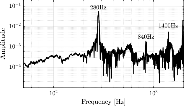
Figure 21: Obtained FRF for the X-bending
11.4 Bending - Y
The setup to measure the Y-bending is shown in Figure 22.
The impact point of the instrumented hammer is located on the back surface of the top interface (on the back of the 2 measurements points).

Figure 22: Y-Bending measurement setup
The data is loaded, and the transfer function from the force to the measured rotation is computed.
bending_Y = load('apa300ml_bending_Y_top.mat');
[G_bending_Y, ~]  = tfestimate(bending_Y.Track1, bending_Y.Track2, win, [], [], 1/Ts);
The results are shown in Figure 23. The main resonance is at 412Hz, and we also see the third “harmonic” at 1220Hz.
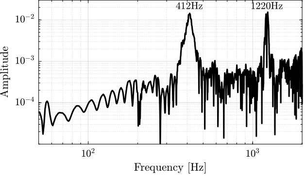
Figure 23: Obtained FRF for the Y-bending
11.5 Torsion - Z
Finally, we measure the Z-torsion resonance as shown in Figure 24.
The excitation is shown on the other side of the APA, on the side to excite the torsion motion.
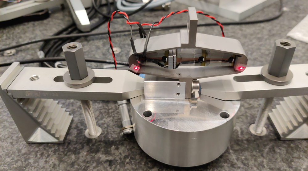
Figure 24: Z-Torsion measurement setup
The data is loaded, and the transfer function computed.
torsion = load('apa300ml_torsion_left.mat');
[G_torsion, ~]  = tfestimate(torsion.Track1, torsion.Track2, win, [], [], 1/Ts);
The results are shown in Figure 25. We observe a first peak at 267Hz, which corresponds to the X-bending mode that was measured at 280Hz. And then a second peak at 415Hz, which corresponds to the X-bending mode that was measured at 412Hz. The mode in pure torsion is probably at higher frequency (peak around 1kHz?).
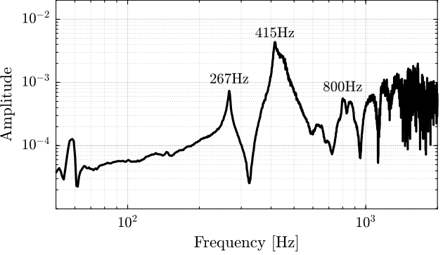
Figure 25: Obtained FRF for the Z-torsion
In order to verify that, the APA is excited on the top part such that the torsion mode should not be excited.
torsion = load('apa300ml_torsion_top.mat');
[G_torsion_top, ~]  = tfestimate(torsion.Track1, torsion.Track2, win, [], [], 1/Ts);
The two FRF are compared in Figure 26. It is clear that the first two modes does not correspond to the torsional mode. Maybe the resonance at 800Hz, or even higher resonances. It is difficult to conclude here.

Figure 26: Obtained FRF for the Z-torsion
11.6 Compare
The three measurements are shown in Figure 27.
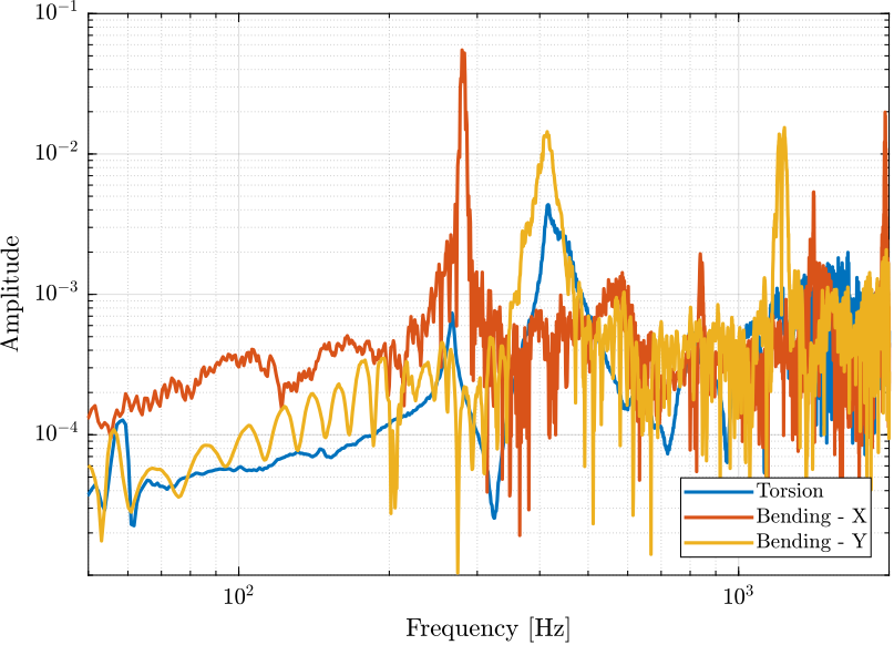
Figure 27: Obtained FRF - Comparison
11.7 Conclusion
When two flexible joints are fixed at each ends of the APA, the APA is mostly in a free/free condition in terms of bending/torsion (the bending/torsional stiffness of the joints being very small).
In the current tests, the APA are in a fixed/free condition. Therefore, it is quite obvious that we measured higher resonance frequencies than what is foreseen for the struts. It is however quite interesting that there is a factor \(\approx \sqrt{2}\) between the two (increased of the stiffness by a factor 2?).
| Mode | Strut Mode | Measured Frequency |
|---|---|---|
| X-Bending | 189Hz | 280Hz |
| Y-Bending | 285Hz | 410Hz |
| Z-Torsion | 400Hz | ? |