Test Bench APA95ML
Table of Contents
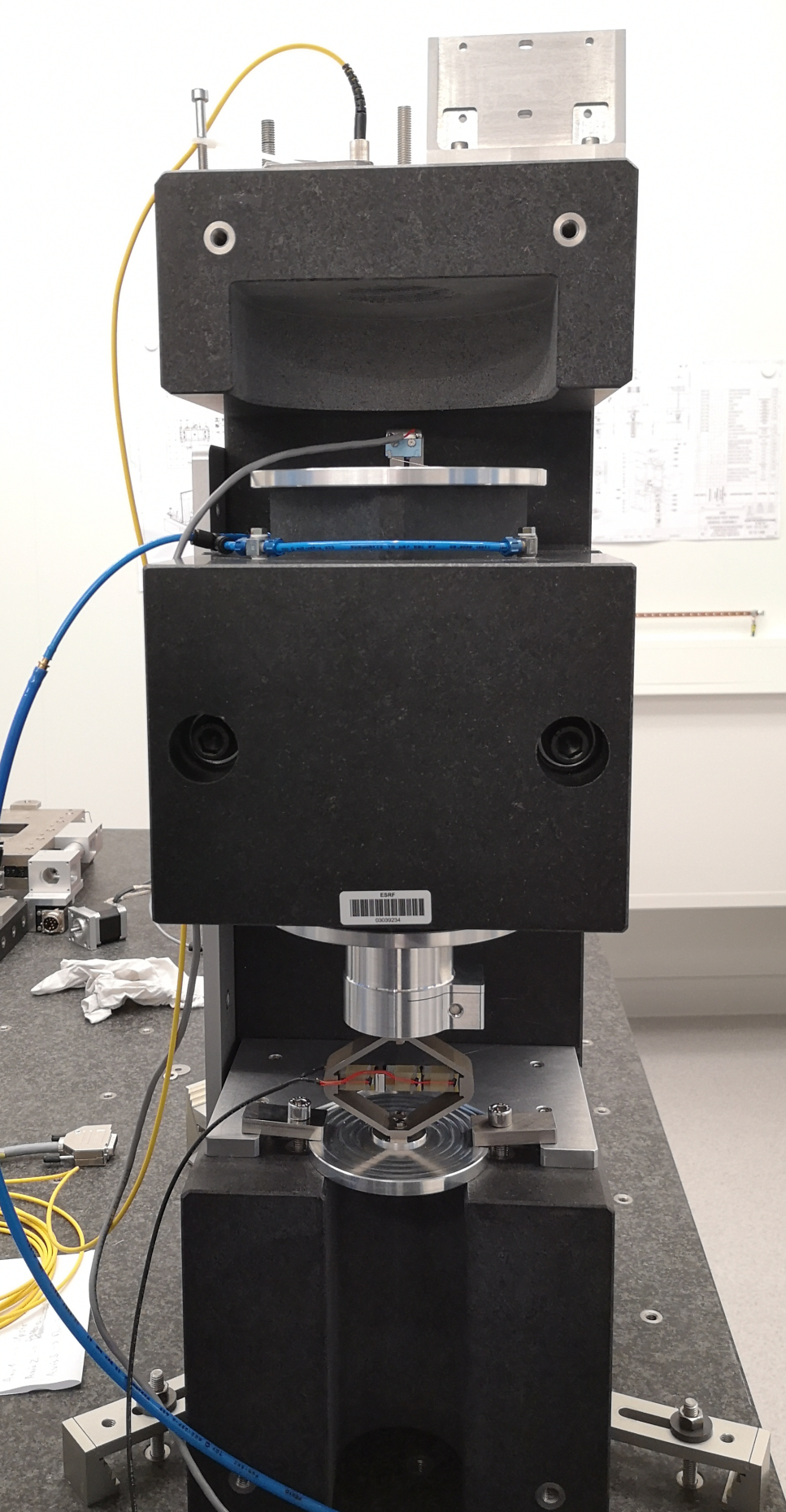
Figure 1: Picture of the Setup
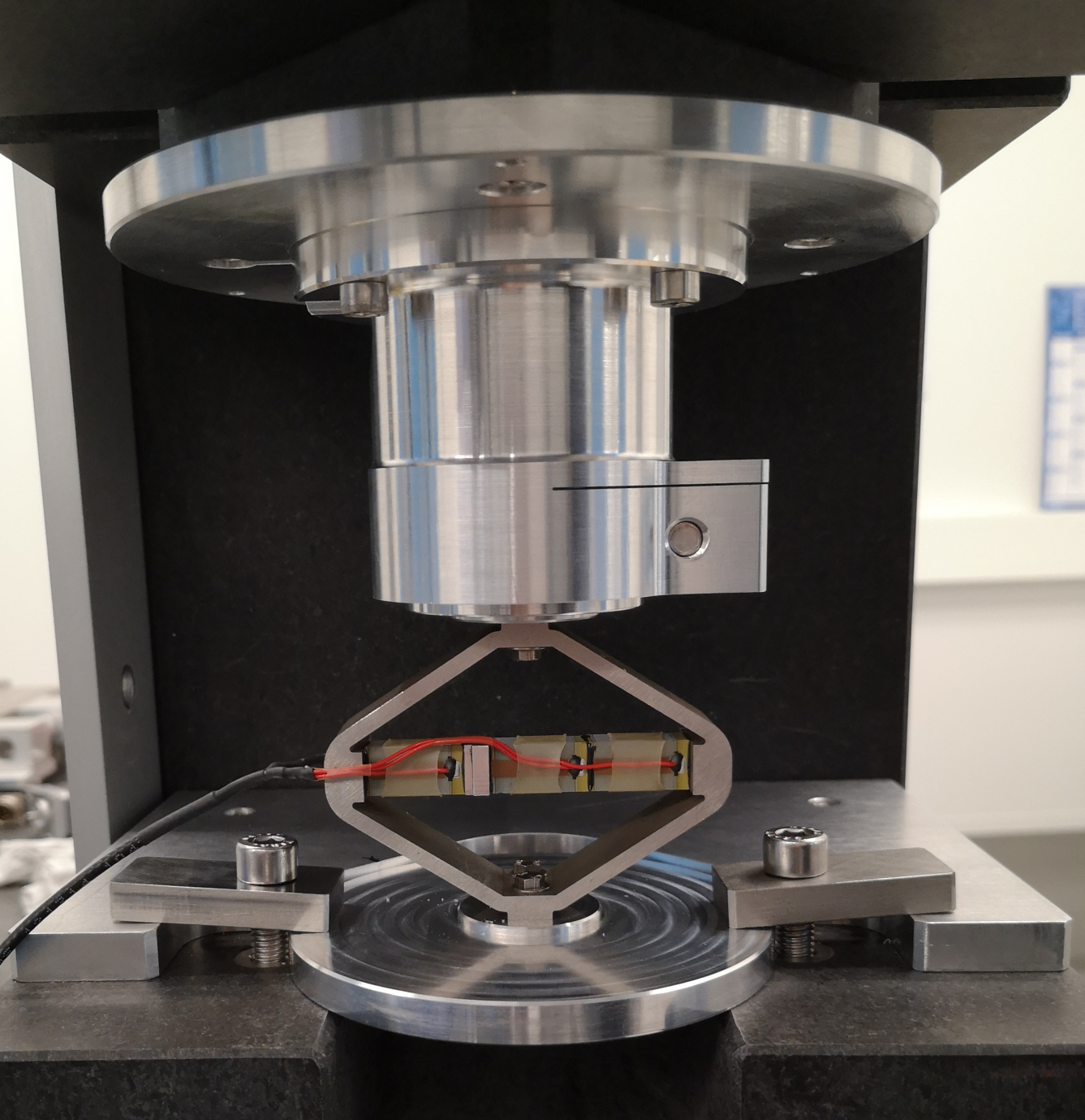
Figure 2: Zoom on the APA
1 Setup
1.1 Parameters
Ts = 1e-4;
1.2 Filter White Noise
Glpf = 1/(1 + s/2/pi/500);

Gz = c2d(Glpf, Ts, 'tustin');
2 Run Experiment and Save Data
2.1 Load Data
data = SimulinkRealTime.utils.getFileScopeData('data/apa95ml.dat').data;
2.2 Save Data
u = data(:, 1); % Input Voltage [V]
y = data(:, 2); % Output Displacement [m]
t = data(:, 3); % Time [s]
save('./mat/huddle_test.mat', 't', 'u', 'y', 'Glpf');
3 Huddle Test
3.1 Time Domain Data
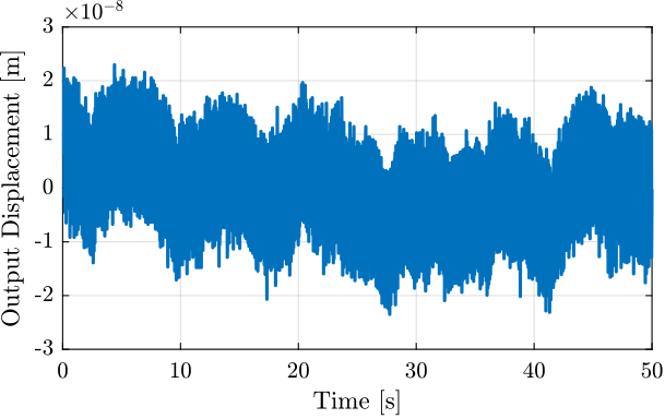
Figure 3: Measurement of the Mass displacement during Huddle Test
3.2 PSD of Measurement Noise
Ts = t(end)/(length(t)-1);
Fs = 1/Ts;

win = hanning(ceil(1*Fs));
[pxx, f] = pwelch(y(1000:end), win, [], [], Fs);

Figure 4: Amplitude Spectral Density of the Displacement during Huddle Test
4 Transfer Function Estimation using the DAC as the driver
4.1 Time Domain Data
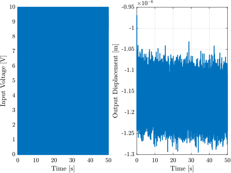
Figure 5: Time domain signals during the test
4.2 Comparison of the PSD with Huddle Test
Ts = t(end)/(length(t)-1);
Fs = 1/Ts;

win = hanning(ceil(1*Fs));
[pxx, f] = pwelch(y, win, [], [], Fs);
[pht, ~] = pwelch(ht.y, win, [], [], Fs);
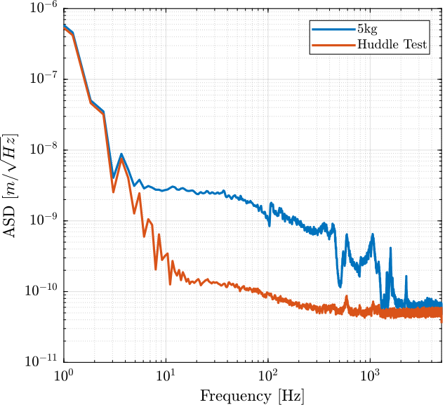
Figure 6: Comparison of the ASD for the identification test and the huddle test
4.3 Compute TF estimate and Coherence
Ts = t(end)/(length(t)-1);
Fs = 1/Ts;
win = hann(ceil(1/Ts));

[tf_est, f] = tfestimate(u, -y, win, [], [], 1/Ts);
[co_est, ~] = mscohere(  u, -y, win, [], [], 1/Ts);

Figure 7: Coherence
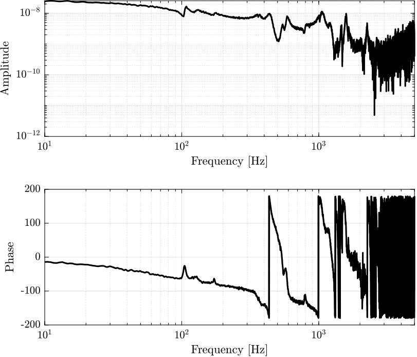
Figure 8: Estimation of the transfer function from input voltage to displacement
4.4 Comparison with the FEM model
load('mat/fem_model_5kg.mat', 'Ghm');

Figure 9: Comparison of the identified transfer function and the one estimated from the FE model
The problem comes from the fact that the piezo is driven directly by the DAC that cannot deliver enought current. In the next section, a current amplifier is used.
5 Transfer Function Estimation using the PI Amplifier
5.1 Comparison of the PSD with Huddle Test
Ts = t(end)/(length(t)-1);
Fs = 1/Ts;

win = hanning(ceil(1*Fs));
[pxx, f] = pwelch(y, win, [], [], Fs);
[pht, ~] = pwelch(ht.y, win, [], [], Fs);
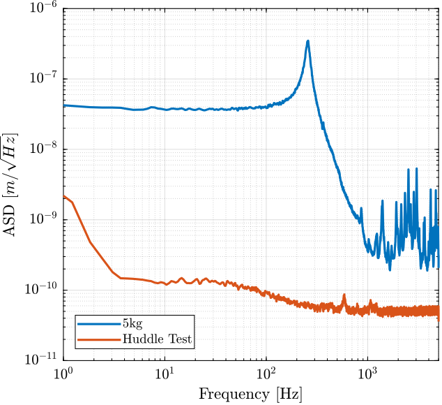
Figure 10: Comparison of the ASD for the identification test and the huddle test
5.2 Compute TF estimate and Coherence
Ts = t(end)/(length(t)-1);
Fs = 1/Ts;
win = hann(ceil(1/Ts));

[tf_est, f] = tfestimate(u,  -y, win, [], [], 1/Ts);
[tf_um , ~] = tfestimate(um, -y, win, [], [], 1/Ts);
[co_est, ~] = mscohere(  um, -y, win, [], [], 1/Ts);

Figure 11: Coherence
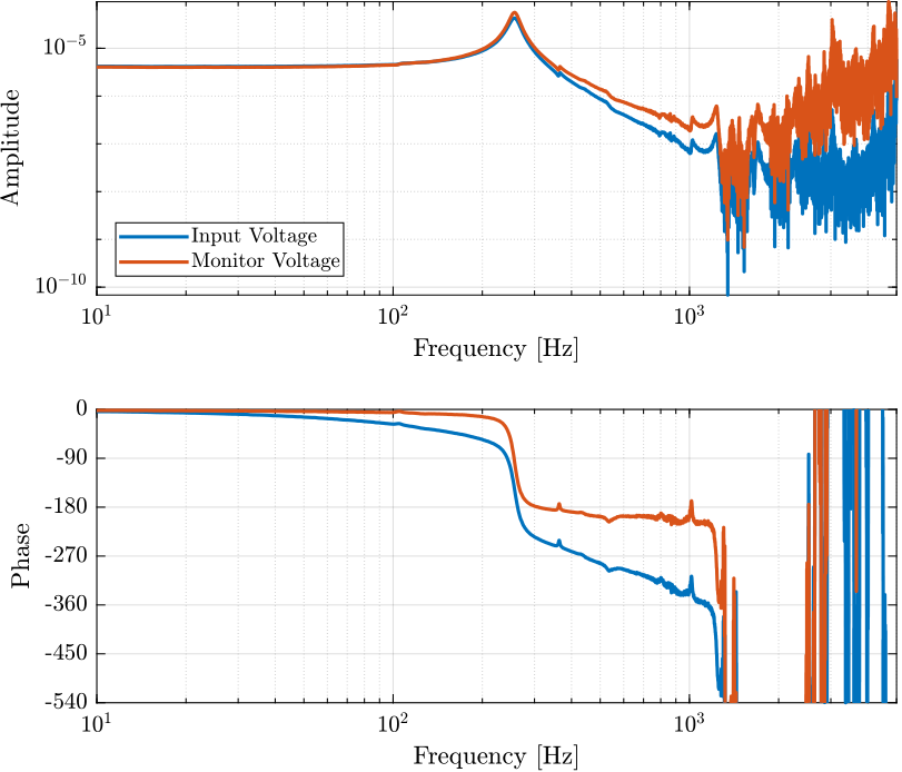
Figure 12: Estimation of the transfer function from input voltage to displacement
5.3 Comparison with the FEM model
load('mat/fem_model_5kg.mat', 'Ghm');

Figure 13: Comparison of the identified transfer function and the one estimated from the FE model
6 Transfer function of the PI Amplifier
6.1 Compute TF estimate and Coherence
Ts = t(end)/(length(t)-1);
Fs = 1/Ts;
The coherence and the transfer function are estimate from the voltage input of the PI amplifier to its voltage inputs.
The coherence is very good as expected (Figure 14).
The transfer function show a low pass filter behavior with a lot of phase drop (Figure 15).
win = hann(ceil(10/Ts));

[tf_est, f] = tfestimate(u, um, win, [], [], 1/Ts);
[co_est, ~] = mscohere(  u, um, win, [], [], 1/Ts);

Figure 14: Coherence
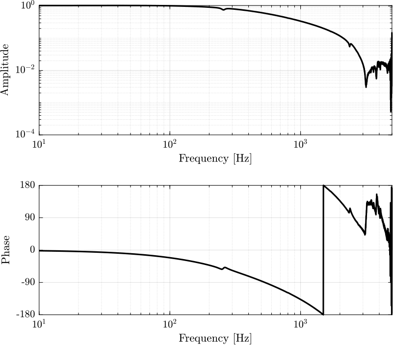
Figure 15: Estimation of the transfer function from input voltage to displacement
The delay can be estimated as follow (in ms):
finddelay(u, um)*(1000*Ts)
0.4
This most probably corresponds to a FIR filter.