Test Bench APA95ML
Table of Contents
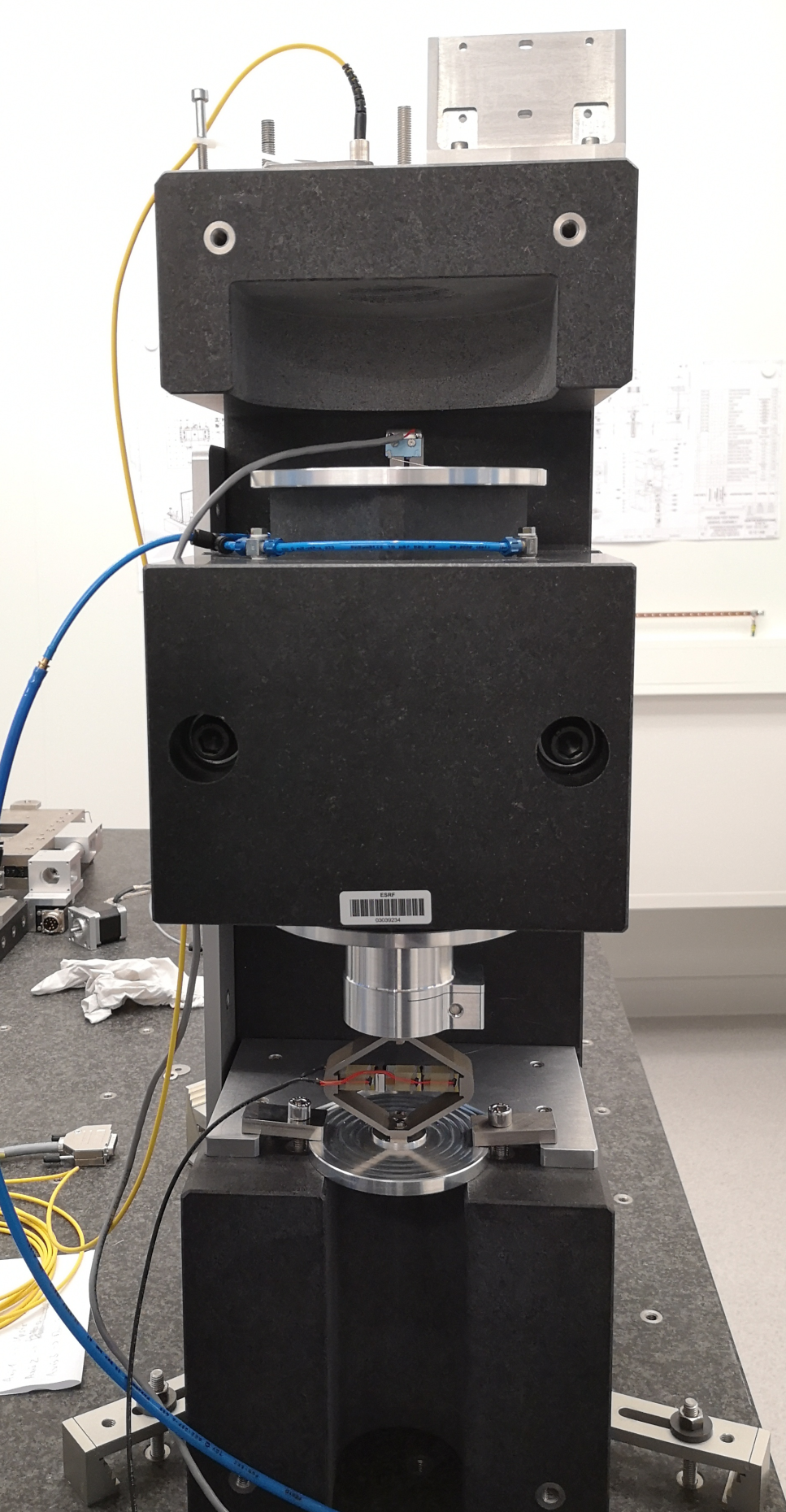
Figure 1: Picture of the Setup
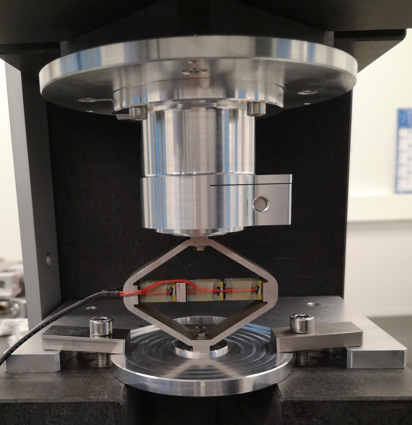
Figure 2: Zoom on the APA
1 Huddle Test
1.1 Time Domain Data
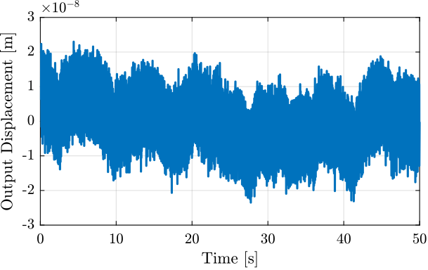
Figure 3: Measurement of the Mass displacement during Huddle Test
1.2 PSD of Measurement Noise
Ts = t(end)/(length(t)-1);
Fs = 1/Ts;

win = hanning(ceil(1*Fs));
[pxx, f] = pwelch(y(1000:end), win, [], [], Fs);
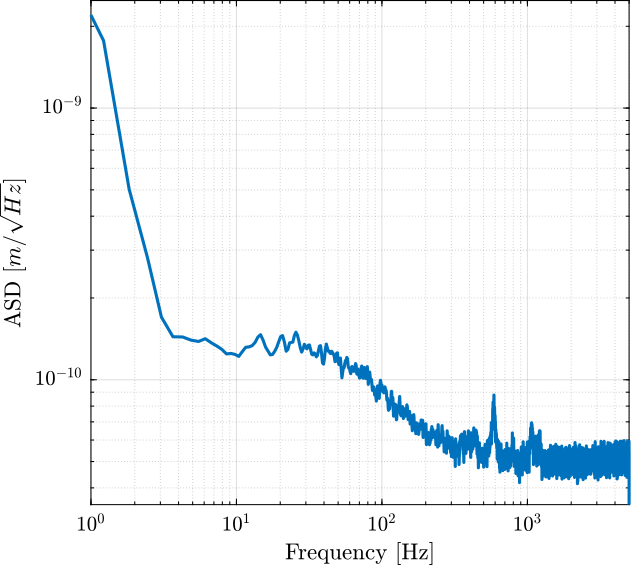
Figure 4: Amplitude Spectral Density of the Displacement during Huddle Test
2 Identification of the dynamics from actuator to displacement
2.1 Load Data
ht = load('huddle_test.mat', 't', 'u', 'y');
load('apa95ml_5kg_Amp_E505.mat', 't', 'u', 'um', 'y');
u  = 10*(u  - mean(u)); % Input Voltage of Piezo [V]
um = 10*(um - mean(um)); % Monitor [V]
y  = y  - mean(y); % Mass displacement [m]

ht.u  = 10*(ht.u  - mean(ht.u));
ht.y  = ht.y  - mean(ht.y);
2.2 Comparison of the PSD with Huddle Test
Ts = t(end)/(length(t)-1);
Fs = 1/Ts;

win = hanning(ceil(1*Fs));
[pxx, f] = pwelch(y, win, [], [], Fs);
[pht, ~] = pwelch(ht.y, win, [], [], Fs);
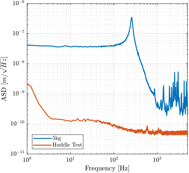
Figure 5: Comparison of the ASD for the identification test and the huddle test
2.3 Compute TF estimate and Coherence
Ts = t(end)/(length(t)-1);
Fs = 1/Ts;
win = hann(ceil(1/Ts));

[tf_est, f] = tfestimate(u,  -y, win, [], [], 1/Ts);
[tf_um , ~] = tfestimate(um, -y, win, [], [], 1/Ts);
[co_est, ~] = mscohere(  um, -y, win, [], [], 1/Ts);
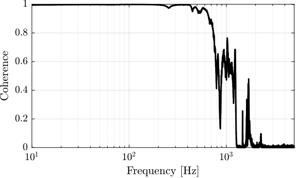
Figure 6: Coherence
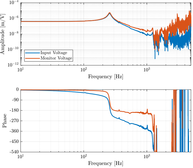
Figure 7: Estimation of the transfer function from input voltage to displacement
2.4 Comparison with the FEM model
load('fem_model_5kg.mat', 'G');
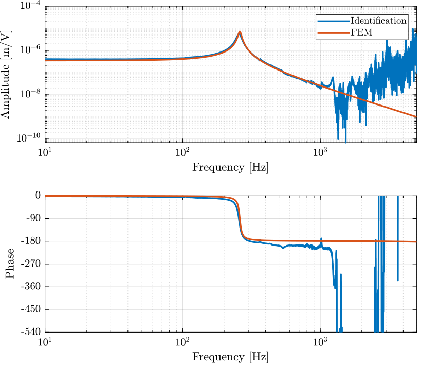
Figure 8: Comparison of the identified transfer function and the one estimated from the FE model
3 Identification of the dynamics from actuator to force sensor
Two measurements are performed:
- Speedgoat DAC => Voltage Amplifier (x20) => 1 Piezo Stack => … => 2 Stacks as Force Sensor (parallel) => Speedgoat ADC
- Speedgoat DAC => Voltage Amplifier (x20) => 2 Piezo Stacks (parallel) => … => 1 Stack as Force Sensor => Speedgoat ADC
The obtained dynamics from force actuator to force sensor are compare with the FEM model.
The data are loaded:
a_ss = load('apa95ml_5kg_1a_2s.mat', 't', 'u', 'y', 'v');
aa_s = load('apa95ml_5kg_2a_1s.mat', 't', 'u', 'y', 'v');
load('G_force_sensor_5kg.mat', 'G');
Let’s use the amplifier gain to obtain the true voltage applied to the actuator stack(s)
The parameters of the piezoelectric stacks are defined below:
d33 = 3e-10; % Strain constant [m/V]
n = 80; % Number of layers per stack
eT = 1.6e-8; % Permittivity under constant stress [F/m]
sD = 2e-11; % Elastic compliance under constant electric displacement [m2/N]
ka = 235e6; % Stack stiffness [N/m]
From the FEM, we construct the transfer function from DAC voltage to ADC voltage.
Gfem_aa_s = exp(-s/1e4)*20*(2*d33*n*ka)*(G(3,1)+G(3,2))*d33/(eT*sD*n);
Gfem_a_ss = exp(-s/1e4)*20*(  d33*n*ka)*(G(3,1)+G(2,1))*d33/(eT*sD*n);
The transfer function from input voltage to output voltage are computed and shown in Figure 9.
Ts = a_ss.t(end)/(length(a_ss.t)-1);
Fs = 1/Ts;

win = hann(ceil(10/Ts));

[tf_a_ss,  f] = tfestimate(a_ss.u, a_ss.v, win, [], [], 1/Ts);
[coh_a_ss, ~] = mscohere(  a_ss.u, a_ss.v, win, [], [], 1/Ts);

[tf_aa_s,  f] = tfestimate(aa_s.u, aa_s.v, win, [], [], 1/Ts);
[coh_aa_s, ~] = mscohere(  aa_s.u, aa_s.v, win, [], [], 1/Ts);
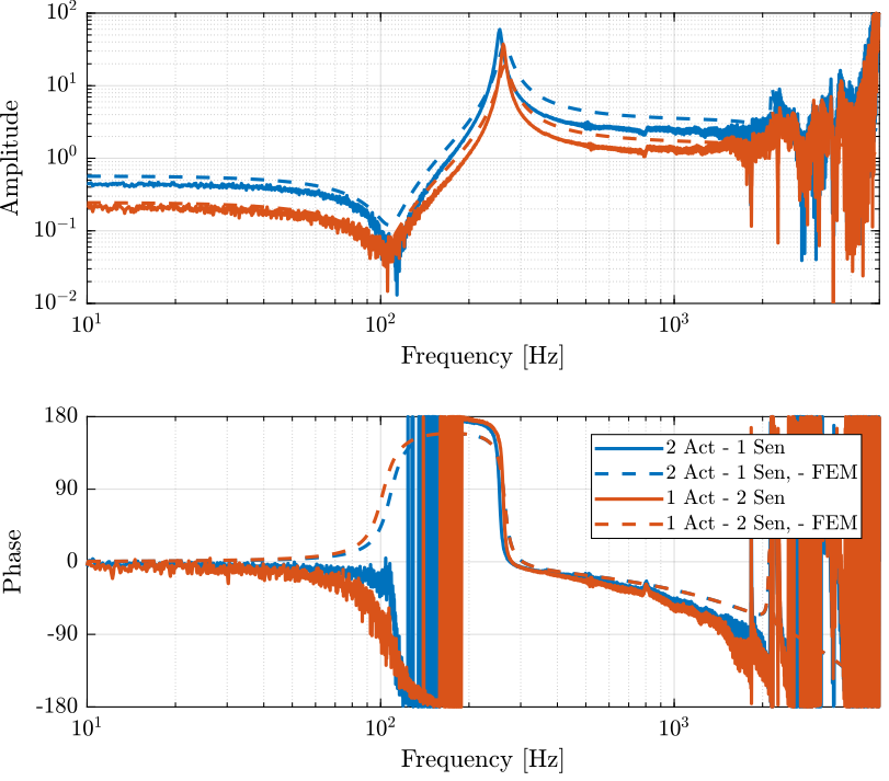
Figure 9: Comparison of the identified dynamics from voltage output to voltage input and the FEM
3.1 System Identification
w_z = 2*pi*111; % Zeros frequency [rad/s]
w_p = 2*pi*255; % Pole frequency [rad/s]
xi_z = 0.05;
xi_p = 0.015;
G_inf = 2;

Gi = G_inf*(s^2 - 2*xi_z*w_z*s + w_z^2)/(s^2 + 2*xi_p*w_p*s + w_p^2);
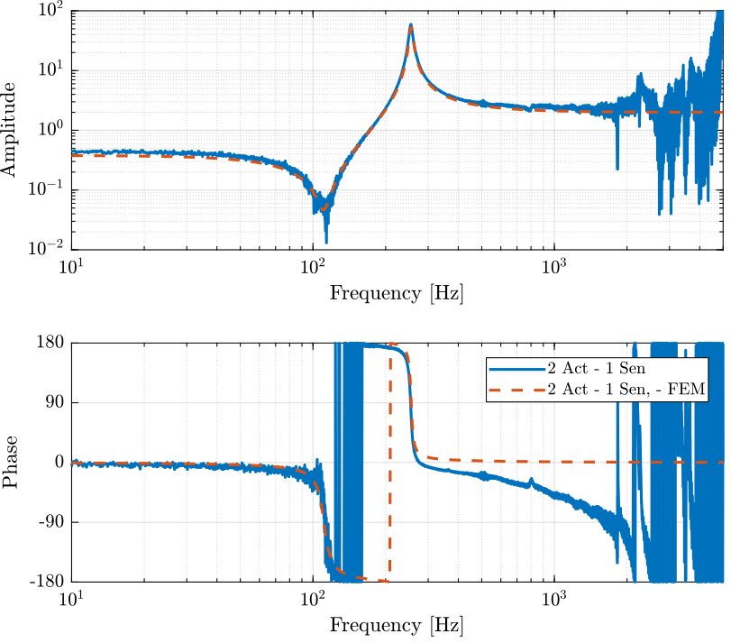
Figure 10: Identification of the IFF plant
3.2 Integral Force Feedback
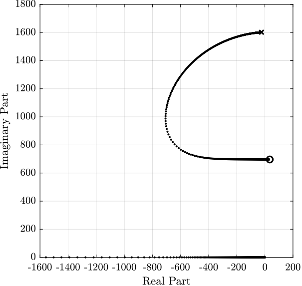
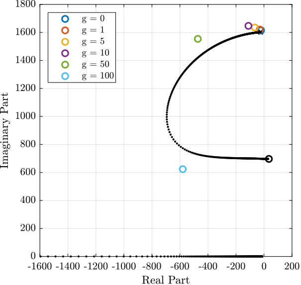
Figure 11: Root Locus for IFF
4 Integral Force Feedback
4.1 First tests with few gains
iff_g10 = load('apa95ml_iff_g10_res.mat', 'u', 't', 'y', 'v');
iff_g100 = load('apa95ml_iff_g100_res.mat', 'u', 't', 'y', 'v');
iff_of = load('apa95ml_iff_off_res.mat', 'u', 't', 'y', 'v');
Ts = 1e-4;
win = hann(ceil(10/Ts));

[tf_iff_g10, f] = tfestimate(iff_g10.u, iff_g10.y, win, [], [], 1/Ts);
[co_iff_g10, ~] = mscohere(iff_g10.u, iff_g10.y, win, [], [], 1/Ts);

[tf_iff_g100, f] = tfestimate(iff_g100.u, iff_g100.y, win, [], [], 1/Ts);
[co_iff_g100, ~] = mscohere(iff_g100.u, iff_g100.y, win, [], [], 1/Ts);

[tf_iff_of, ~] = tfestimate(iff_of.u, iff_of.y, win, [], [], 1/Ts);
[co_iff_of, ~] = mscohere(iff_of.u, iff_of.y, win, [], [], 1/Ts);
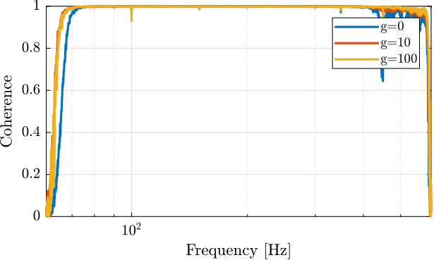
Figure 12: Coherence
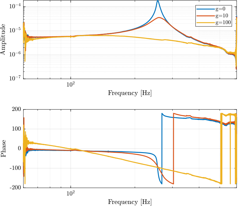
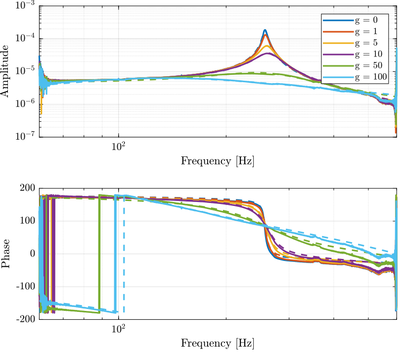
Figure 13: Bode plot for different values of IFF gain
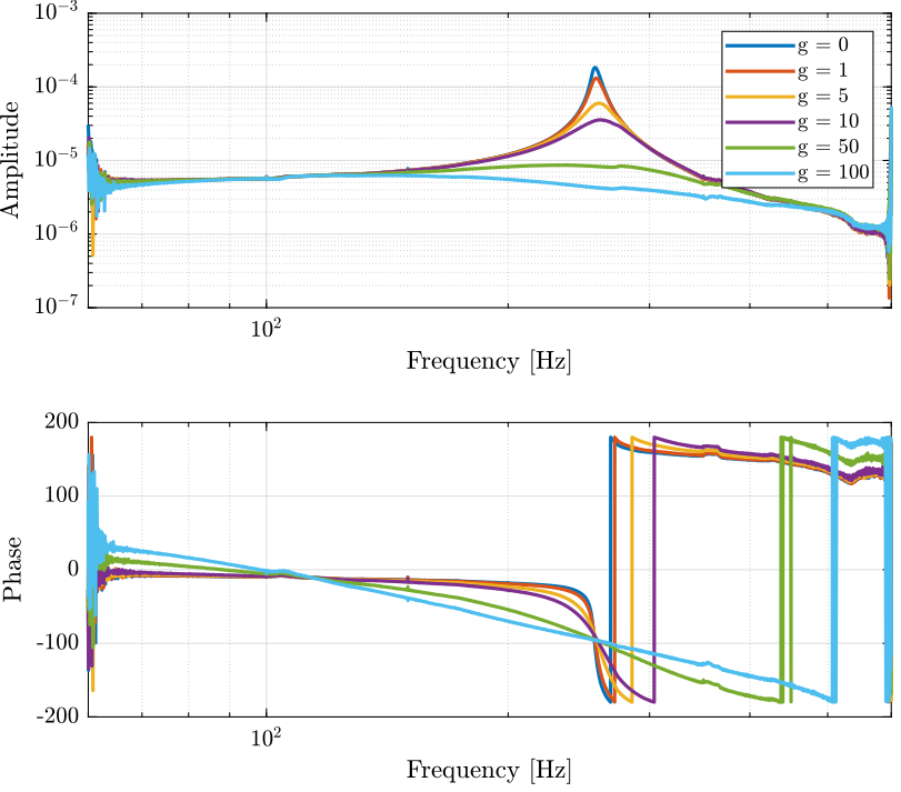
4.2 Second test with many Gains
load('apa95ml_iff_test.mat', 'results');
Ts = 1e-4;
win = hann(ceil(10/Ts));
tf_iff = {zeros(1, length(results))};
co_iff = {zeros(1, length(results))};
g_iff = [0, 1, 5, 10, 50, 100];

for i=1:length(results)
    [tf_est, f] = tfestimate(results{i}.u, results{i}.y, win, [], [], 1/Ts);
    [co_est, ~] = mscohere(results{i}.u, results{i}.y, win, [], [], 1/Ts);

    tf_iff(i) = {tf_est};
    co_iff(i) = {co_est};
end
G_id = {zeros(1,length(results))};

f_start = 70; % [Hz]
f_end = 500; % [Hz]

for i = 1:length(results)
    tf_id = tf_iff{i}(sum(f<f_start):length(f)-sum(f>f_end));
    f_id = f(sum(f<f_start):length(f)-sum(f>f_end));

    gfr = idfrd(tf_id, 2*pi*f_id, Ts);
    G_id(i) = {procest(gfr,'P2UDZ')};
end