Test Bench APA95ML
Table of Contents
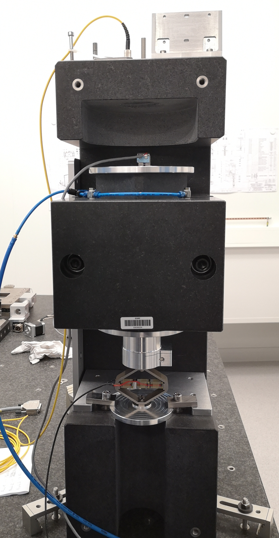
Figure 1: Picture of the Setup
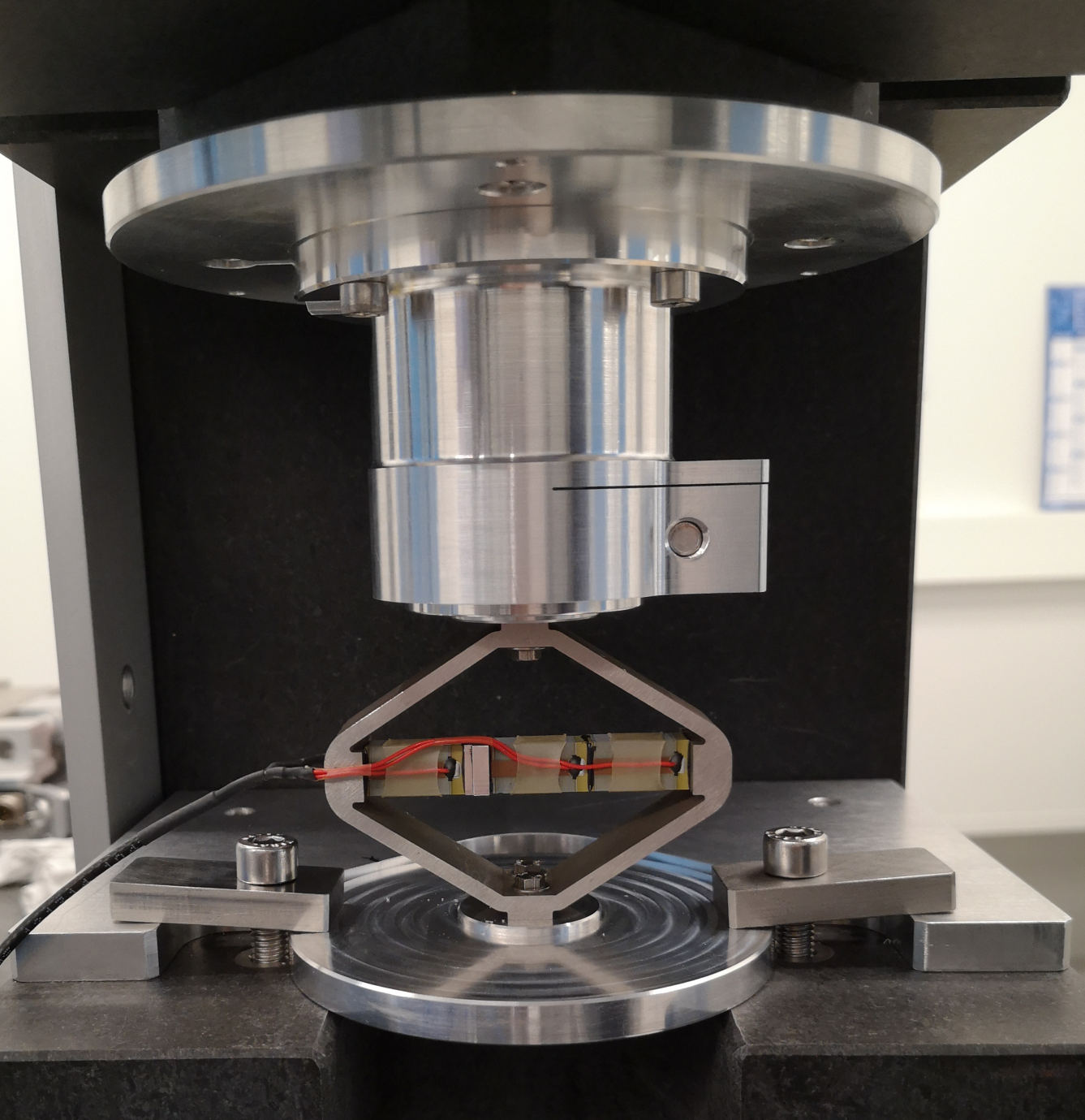
Figure 2: Zoom on the APA
1 Setup
1.1 Parameters
Ts = 1e-4;
1.2 Filter White Noise
Glpf = 1/(1 + s/2/pi/500);

Gz = c2d(Glpf, Ts, 'tustin');
2 Run Experiment and Save Data
2.1 Load Data
data = SimulinkRealTime.utils.getFileScopeData('data/apa95ml.dat').data;
2.2 Save Data
u = data(:, 1); % Input Voltage [V]
y = data(:, 2); % Output Displacement [m]
t = data(:, 3); % Time [s]
save('./mat/huddle_test.mat', 't', 'u', 'y', 'Glpf');
3 Huddle Test
3.1 Time Domain Data
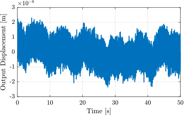
Figure 3: Measurement of the Mass displacement during Huddle Test
3.2 PSD of Measurement Noise
Ts = t(end)/(length(t)-1);
Fs = 1/Ts;

win = hanning(ceil(1*Fs));
[pxx, f] = pwelch(y(1000:end), win, [], [], Fs);
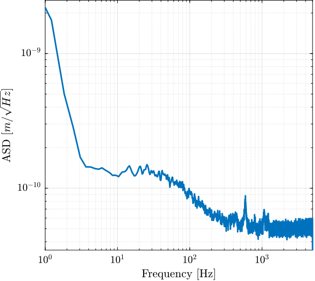
Figure 4: Amplitude Spectral Density of the Displacement during Huddle Test
4 Transfer Function Estimation using the DAC as the driver
Results presented in this sections are wrong as the ADC cannot deliver enought current to the piezoelectric actuator.
4.1 Time Domain Data
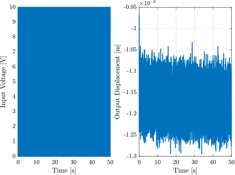
Figure 5: Time domain signals during the test
4.2 Comparison of the PSD with Huddle Test
Ts = t(end)/(length(t)-1);
Fs = 1/Ts;

win = hanning(ceil(1*Fs));
[pxx, f] = pwelch(y, win, [], [], Fs);
[pht, ~] = pwelch(ht.y, win, [], [], Fs);
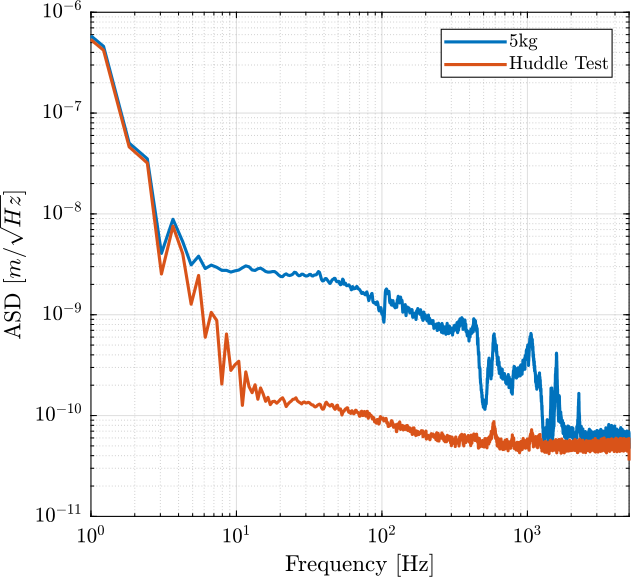
Figure 6: Comparison of the ASD for the identification test and the huddle test
4.3 Compute TF estimate and Coherence
Ts = t(end)/(length(t)-1);
Fs = 1/Ts;
win = hann(ceil(1/Ts));

[tf_est, f] = tfestimate(u, -y, win, [], [], 1/Ts);
[co_est, ~] = mscohere(  u, -y, win, [], [], 1/Ts);
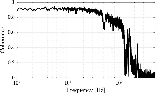
Figure 7: Coherence
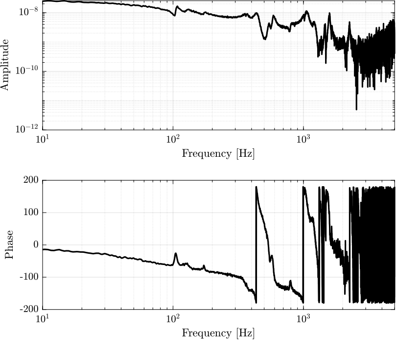
Figure 8: Estimation of the transfer function from input voltage to displacement
4.4 Comparison with the FEM model
load('mat/fem_model_5kg.mat', 'Ghm');
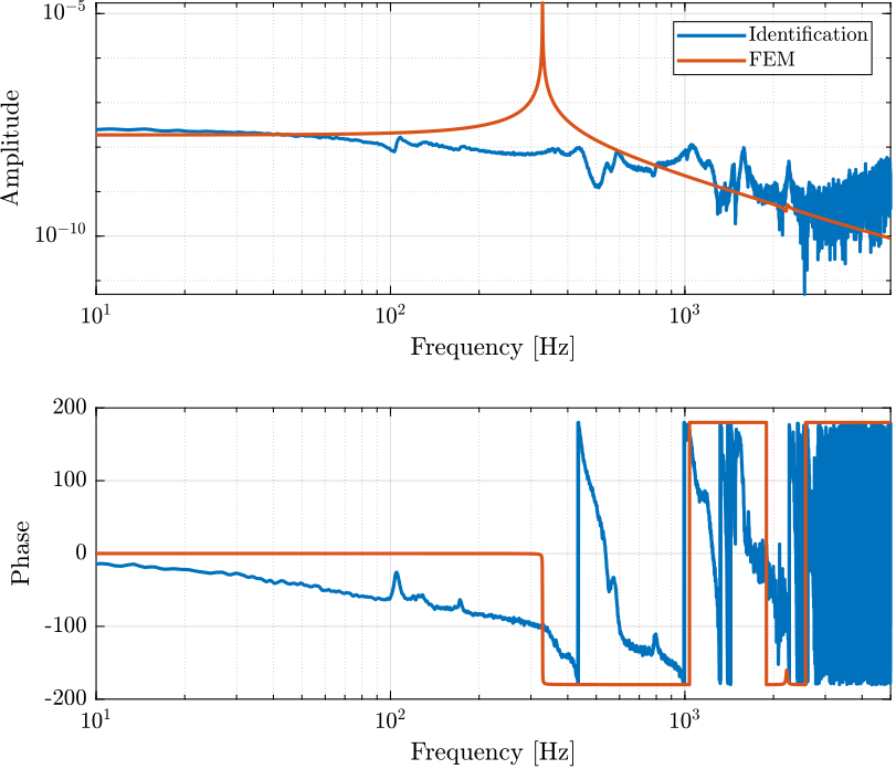
Figure 9: Comparison of the identified transfer function and the one estimated from the FE model
The problem comes from the fact that the piezo is driven directly by the DAC that cannot deliver enought current. In the next section, a current amplifier is used.
5 Transfer Function Estimation using the PI Amplifier
5.1 Load Data
ht = load('./mat/huddle_test.mat', 't', 'u', 'y');
load('./mat/apa95ml_5kg_Amp_E505.mat', 't', 'u', 'um', 'y');
u  = 10*(u  - mean(u)); % Input Voltage of Piezo [V]
um = 10*(um - mean(um)); % Monitor [V]
y  = y  - mean(y); % Mass displacement [m]

ht.u  = 10*(ht.u  - mean(ht.u));
ht.y  = ht.y  - mean(ht.y);
5.2 Comparison of the PSD with Huddle Test
Ts = t(end)/(length(t)-1);
Fs = 1/Ts;

win = hanning(ceil(1*Fs));
[pxx, f] = pwelch(y, win, [], [], Fs);
[pht, ~] = pwelch(ht.y, win, [], [], Fs);
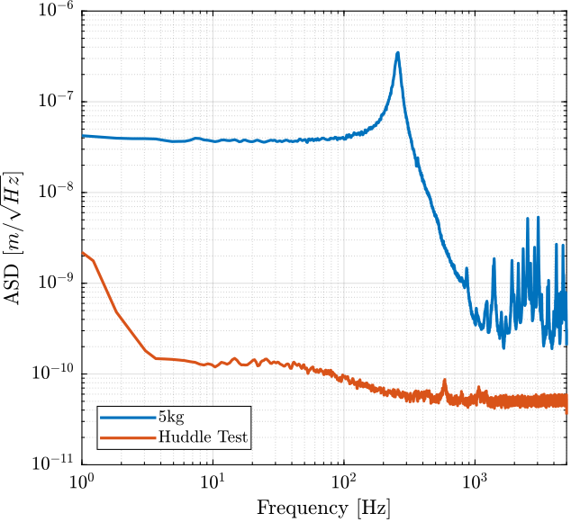
Figure 10: Comparison of the ASD for the identification test and the huddle test
5.3 Compute TF estimate and Coherence
Ts = t(end)/(length(t)-1);
Fs = 1/Ts;
win = hann(ceil(1/Ts));

[tf_est, f] = tfestimate(u,  -y, win, [], [], 1/Ts);
[tf_um , ~] = tfestimate(um, -y, win, [], [], 1/Ts);
[co_est, ~] = mscohere(  um, -y, win, [], [], 1/Ts);
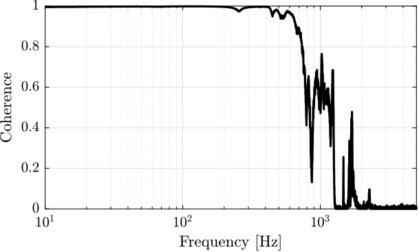
Figure 11: Coherence
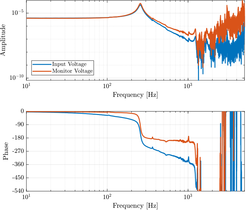
Figure 12: Estimation of the transfer function from input voltage to displacement
5.4 Comparison with the FEM model
load('mat/fem_model_5kg.mat', 'G');
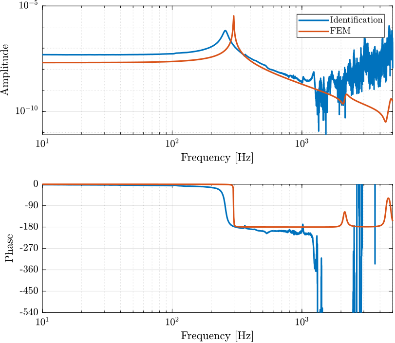
Figure 13: Comparison of the identified transfer function and the one estimated from the FE model
6 Transfer function from force actuator to force sensor
Two measurements are performed:
- Speedgoat DAC => Voltage Amplifier (x20) => 1 Piezo Stack => … => 2 Stacks as Force Sensor (parallel) => Speedgoat ADC
- Speedgoat DAC => Voltage Amplifier (x20) => 2 Piezo Stacks (parallel) => … => 1 Stack as Force Sensor => Speedgoat ADC
The obtained dynamics from force actuator to force sensor are compare with the FEM model.
The data are loaded:
a_ss = load('mat/apa95ml_5kg_1a_2s.mat', 't', 'u', 'y', 'v');
aa_s = load('mat/apa95ml_5kg_2a_1s.mat', 't', 'u', 'y', 'v');
load('mat/G_force_sensor_5kg.mat', 'G');
Let’s use the amplifier gain to obtain the true voltage applied to the actuator stack(s)
The parameters of the piezoelectric stacks are defined below:
d33 = 3e-10; % Strain constant [m/V]
n = 80; % Number of layers per stack
eT = 1.6e-8; % Permittivity under constant stress [F/m]
sD = 2e-11; % Elastic compliance under constant electric displacement [m2/N]
ka = 235e6; % Stack stiffness [N/m]
From the FEM, we construct the transfer function from DAC voltage to ADC voltage.
Gfem_aa_s = exp(-s/1e4)*20*(2*d33*n*ka)*(G(3,1)+G(3,2))*d33/(eT*sD*n);
Gfem_a_ss = exp(-s/1e4)*20*(  d33*n*ka)*(G(3,1)+G(2,1))*d33/(eT*sD*n);
The transfer function from input voltage to output voltage are computed and shown in Figure 14.
Ts = a_ss.t(end)/(length(a_ss.t)-1);
Fs = 1/Ts;

win = hann(ceil(10/Ts));

[tf_a_ss,  f] = tfestimate(a_ss.u, a_ss.v, win, [], [], 1/Ts);
[coh_a_ss, ~] = mscohere(  a_ss.u, a_ss.v, win, [], [], 1/Ts);

[tf_aa_s,  f] = tfestimate(aa_s.u, aa_s.v, win, [], [], 1/Ts);
[coh_aa_s, ~] = mscohere(  aa_s.u, aa_s.v, win, [], [], 1/Ts);
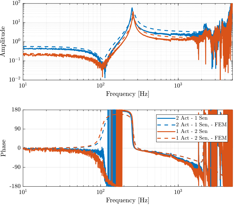
Figure 14: Comparison of the identified dynamics from voltage output to voltage input and the FEM
6.1 System Identification
w_z = 2*pi*111; % Zeros frequency [rad/s]
w_p = 2*pi*255; % Pole frequency [rad/s]
xi_z = 0.05;
xi_p = 0.015;
G_inf = 2;

Gi = G_inf*(s^2 - 2*xi_z*w_z*s + w_z^2)/(s^2 + 2*xi_p*w_p*s + w_p^2);
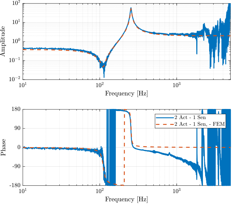
Figure 15: Identification of the IFF plant
6.2 Integral Force Feedback
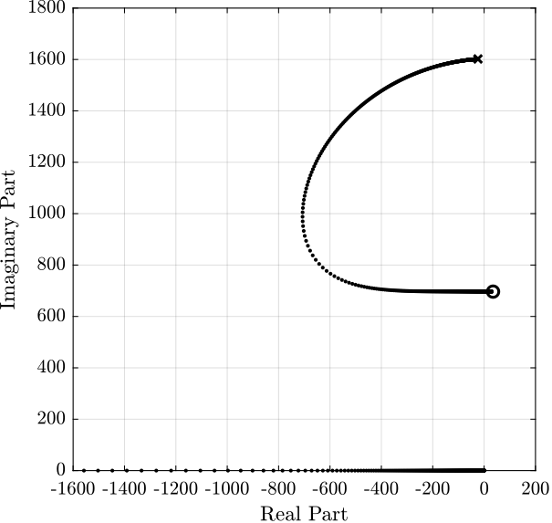
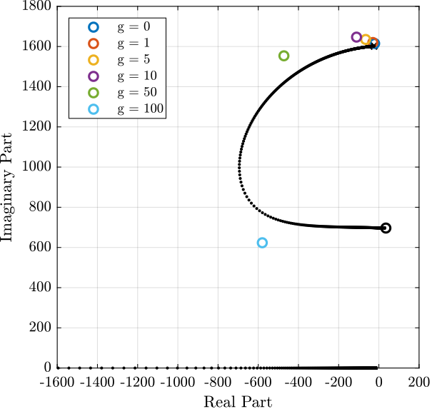
Figure 16: Root Locus for IFF
7 IFF Tests
7.1 First tests with few gains
iff_g10 = load('./mat/apa95ml_iff_g10_res.mat', 'u', 't', 'y', 'v');
iff_g100 = load('./mat/apa95ml_iff_g100_res.mat', 'u', 't', 'y', 'v');
iff_of = load('./mat/apa95ml_iff_off_res.mat', 'u', 't', 'y', 'v');
Ts = 1e-4;
win = hann(ceil(10/Ts));

[tf_iff_g10, f] = tfestimate(iff_g10.u, iff_g10.y, win, [], [], 1/Ts);
[co_iff_g10, ~] = mscohere(iff_g10.u, iff_g10.y, win, [], [], 1/Ts);

[tf_iff_g100, f] = tfestimate(iff_g100.u, iff_g100.y, win, [], [], 1/Ts);
[co_iff_g100, ~] = mscohere(iff_g100.u, iff_g100.y, win, [], [], 1/Ts);

[tf_iff_of, ~] = tfestimate(iff_of.u, iff_of.y, win, [], [], 1/Ts);
[co_iff_of, ~] = mscohere(iff_of.u, iff_of.y, win, [], [], 1/Ts);
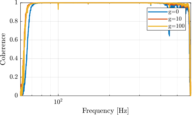
Figure 17: Coherence
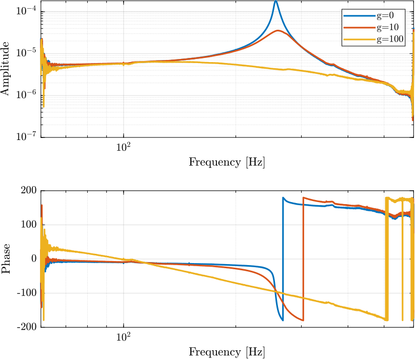
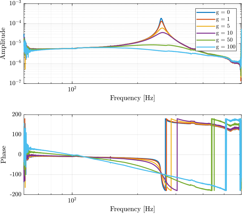
Figure 18: Bode plot for different values of IFF gain
7.2 Second test with many Gains
load('./mat/apa95ml_iff_test.mat', 'results');
Ts = 1e-4;
win = hann(ceil(10/Ts));
tf_iff = {zeros(1, length(results))};
co_iff = {zeros(1, length(results))};
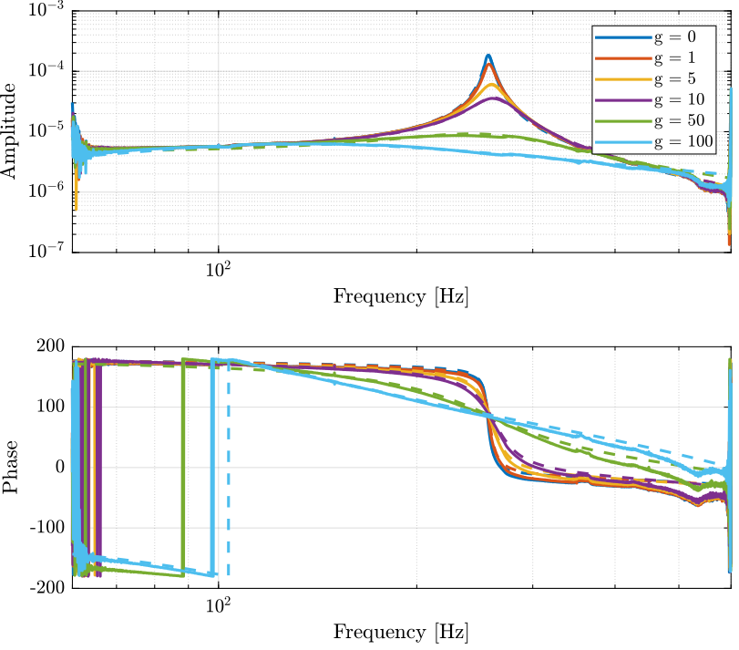
g_iff = [0, 1, 5, 10, 50, 100];

for i=1:length(results)
    [tf_est, f] = tfestimate(results{i}.u, results{i}.y, win, [], [], 1/Ts);
    [co_est, ~] = mscohere(results{i}.u, results{i}.y, win, [], [], 1/Ts);

    tf_iff(i) = {tf_est};
    co_iff(i) = {co_est};
end
G_id = {zeros(1,length(results))};

f_start = 70; % [Hz]
f_end = 500; % [Hz]

for i = 1:length(results)
    tf_id = tf_iff{i}(sum(f<f_start):length(f)-sum(f>f_end));
    f_id = f(sum(f<f_start):length(f)-sum(f>f_end));

    gfr = idfrd(tf_id, 2*pi*f_id, Ts);
    G_id(i) = {procest(gfr,'P2UDZ')};
end
