SVD Control

1. Gravimeter - Simscape Model
- 1.1. Simulink
2. Stewart Platform - Simscape Model
3. Stewart Platform - Analytical Model

1 Gravimeter - Simscape Model

1.1 Simulink

open('gravimeter.slx')

%% Name of the Simulink File
mdl = 'gravimeter';

%% Input/Output definition
clear io; io_i = 1;
io(io_i) = linio([mdl, '/F1'], 1, 'openinput');  io_i = io_i + 1;
io(io_i) = linio([mdl, '/F2'], 1, 'openinput');  io_i = io_i + 1;
io(io_i) = linio([mdl, '/F3'], 1, 'openinput');  io_i = io_i + 1;
io(io_i) = linio([mdl, '/Acc_side'], 1, 'openoutput'); io_i = io_i + 1;
io(io_i) = linio([mdl, '/Acc_side'], 2, 'openoutput'); io_i = io_i + 1;
io(io_i) = linio([mdl, '/Acc_top'], 1, 'openoutput'); io_i = io_i + 1;
io(io_i) = linio([mdl, '/Acc_top'], 2, 'openoutput'); io_i = io_i + 1;

G = linearize(mdl, io);
G.InputName  = {'F1', 'F2', 'F3'};
G.OutputName = {'Ax1', 'Az1', 'Ax2', 'Az2'};

The plant as 6 states as expected (2 translations + 1 rotation)

size(G)

State-space model with 4 outputs, 3 inputs, and 6 states.

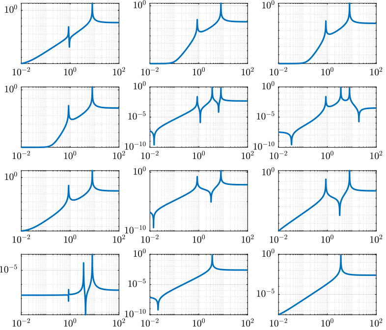
Figure 1: Open Loop Transfer Function from 3 Actuators to 4 Accelerometers

2 Stewart Platform - Simscape Model

2.1 Jacobian

First, the position of the “joints” (points of force application) are estimated and the Jacobian computed.

open('stewart_platform/drone_platform_jacobian.slx');

sim('drone_platform_jacobian');

Aa = [a1.Data(1,:);
      a2.Data(1,:);
      a3.Data(1,:);
      a4.Data(1,:);
      a5.Data(1,:);
      a6.Data(1,:)]';

Ab = [b1.Data(1,:);
      b2.Data(1,:);
      b3.Data(1,:);
      b4.Data(1,:);
      b5.Data(1,:);
      b6.Data(1,:)]';

As = (Ab - Aa)./vecnorm(Ab - Aa);

l = vecnorm(Ab - Aa)';

J = [As' , cross(Ab, As)'];

save('./jacobian.mat', 'Aa', 'Ab', 'As', 'l', 'J');

2.2 Simscape Model

open('stewart_platform/drone_platform.slx');

Definition of spring parameters

kx = 50; % [N/m]
ky = 50;
kz = 50;

cx = 0.025; % [Nm/rad]
cy = 0.025;
cz = 0.025;

We load the Jacobian.

load('./jacobian.mat', 'Aa', 'Ab', 'As', 'l', 'J');

2.3 Identification of the plant

The dynamics is identified from forces applied by each legs to the measured acceleration of the top platform.

%% Name of the Simulink File
mdl = 'drone_platform';

%% Input/Output definition
clear io; io_i = 1;
io(io_i) = linio([mdl, '/Dw'],              1, 'openinput');  io_i = io_i + 1;
io(io_i) = linio([mdl, '/u'],               1, 'openinput');  io_i = io_i + 1;
io(io_i) = linio([mdl, '/Inertial Sensor'], 1, 'openoutput'); io_i = io_i + 1;

G = linearize(mdl, io);
G.InputName  = {'Dwx', 'Dwy', 'Dwz', 'Rwx', 'Rwy', 'Rwz', ...
                'F1', 'F2', 'F3', 'F4', 'F5', 'F6'};
G.OutputName = {'Ax', 'Ay', 'Az', 'Arx', 'Ary', 'Arz'};

There are 24 states (6dof for the bottom platform + 6dof for the top platform).

size(G)

State-space model with 6 outputs, 12 inputs, and 24 states.

% G = G*blkdiag(inv(J), eye(6));
% G.InputName  = {'Dw1', 'Dw2', 'Dw3', 'Dw4', 'Dw5', 'Dw6', ...
%                 'F1', 'F2', 'F3', 'F4', 'F5', 'F6'};

Thanks to the Jacobian, we compute the transfer functions in the frame of the legs and in an inertial frame.

Gx = G*blkdiag(eye(6), inv(J'));
Gx.InputName  = {'Dwx', 'Dwy', 'Dwz', 'Rwx', 'Rwy', 'Rwz', ...
                 'Fx', 'Fy', 'Fz', 'Mx', 'My', 'Mz'};

Gl = J*G;
Gl.OutputName  = {'A1', 'A2', 'A3', 'A4', 'A5', 'A6'};

2.4 Obtained Dynamics

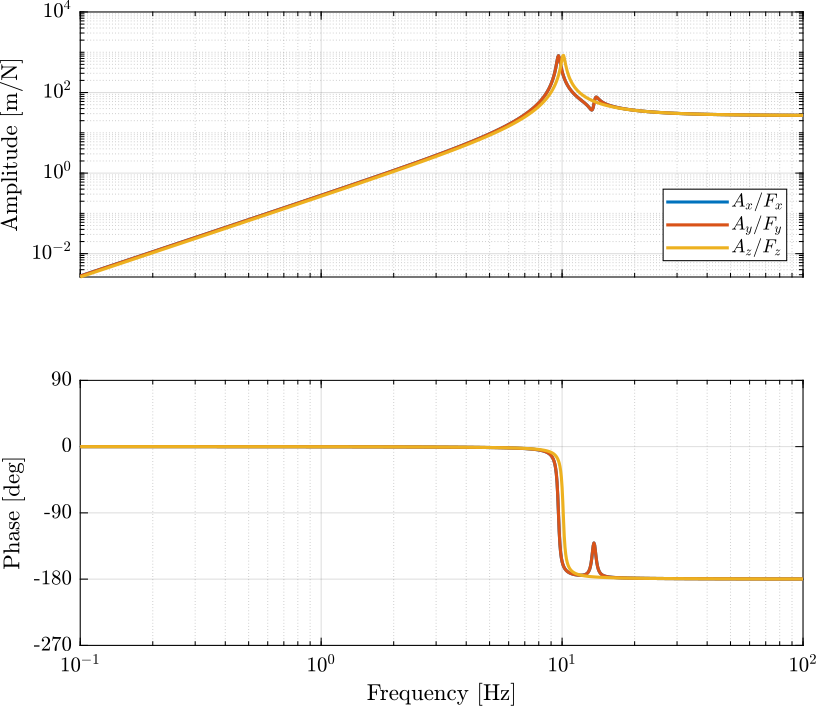
Figure 2: Stewart Platform Plant from forces applied by the legs to the acceleration of the platform

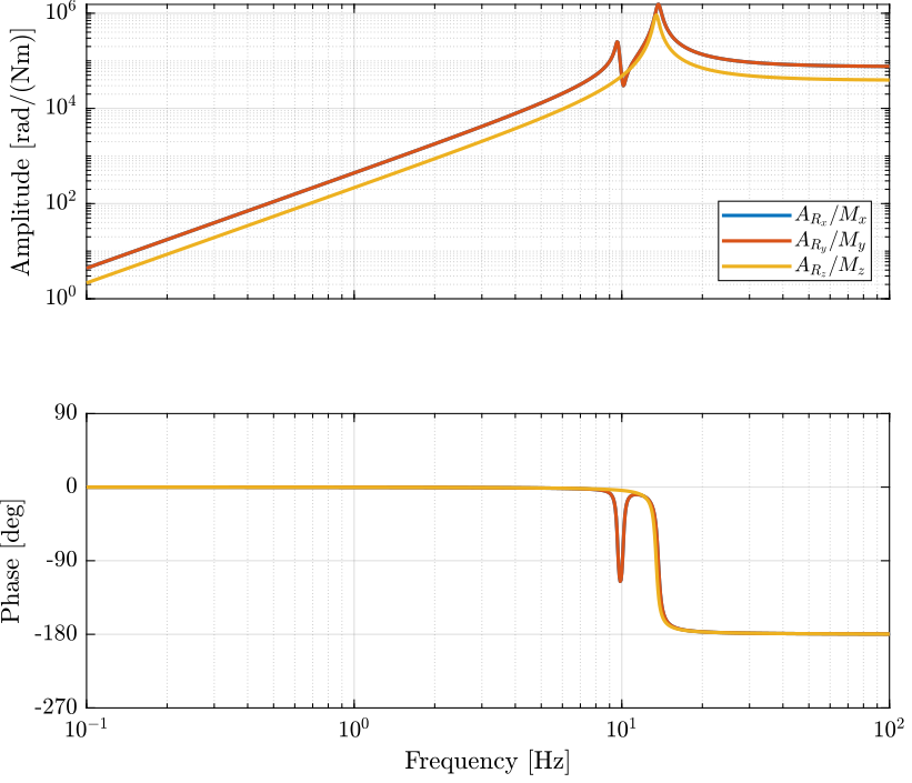
Figure 3: Stewart Platform Plant from torques applied by the legs to the angular acceleration of the platform

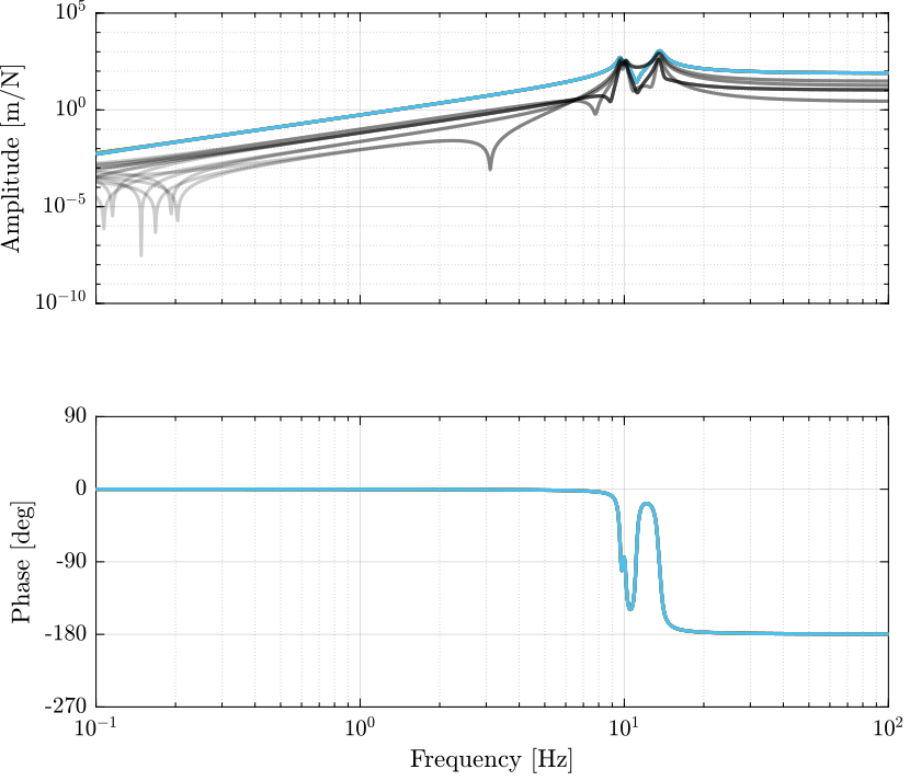
Figure 4: Stewart Platform Plant from forces applied by the legs to displacement of the legs

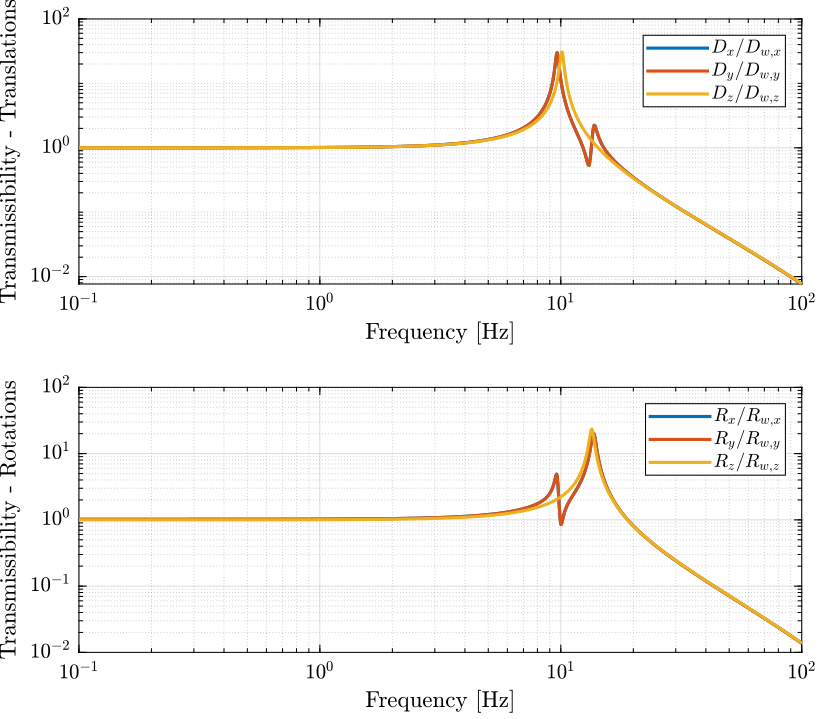
Figure 5: Transmissibility

2.5 Real Approximation of \(G\) at the decoupling frequency

Let’s compute a real approximation of the complex matrix \(H_1\) which corresponds to the the transfer function \(G_c(j\omega_c)\) from forces applied by the actuators to the measured acceleration of the top platform evaluated at the frequency \(\omega_c\).

wc = 2*pi*20; % Decoupling frequency [rad/s]

Gc = G({'Ax', 'Ay', 'Az', 'Arx', 'Ary', 'Arz'}, ...
       {'F1', 'F2', 'F3', 'F4', 'F5', 'F6'}); % Transfer function to find a real approximation

H1 = evalfr(Gc, j*wc);

The real approximation is computed as follows:

D = pinv(real(H1'*H1));
H1 = inv(D*real(H1'*diag(exp(j*angle(diag(H1*D*H1.'))/2))));

2.6 Verification of the decoupling using the “Gershgorin Radii”

First, the Singular Value Decomposition of \(H_1\) is performed: \[ H_1 = U \Sigma V^H \]

[U,S,V] = svd(H1);

Then, the “Gershgorin Radii” is computed for the plant \(G_c(s)\) and the “SVD Decoupled Plant” \(G_d(s)\): \[ G_d(s) = U^T G_c(s) V \]

This is computed over the following frequencies.

freqs = logspace(-2, 2, 1000); % [Hz]

Gershgorin Radii for the coupled plant:

Gr_coupled = zeros(length(freqs), size(Gc,2));

H = abs(squeeze(freqresp(Gc, freqs, 'Hz')));
for out_i = 1:size(Gc,2)
    Gr_coupled(:, out_i) = squeeze((sum(H(out_i,:,:)) - H(out_i,out_i,:))./H(out_i, out_i, :));
end

Gershgorin Radii for the decoupled plant using SVD:

Gd = U'*Gc*V;
Gr_decoupled = zeros(length(freqs), size(Gd,2));

H = abs(squeeze(freqresp(Gd, freqs, 'Hz')));
for out_i = 1:size(Gd,2)
    Gr_decoupled(:, out_i) = squeeze((sum(H(out_i,:,:)) - H(out_i,out_i,:))./H(out_i, out_i, :));
end

Gershgorin Radii for the decoupled plant using the Jacobian:

Gj = Gc*inv(J');
Gr_jacobian = zeros(length(freqs), size(Gj,2));

H = abs(squeeze(freqresp(Gj, freqs, 'Hz')));

for out_i = 1:size(Gj,2)
    Gr_jacobian(:, out_i) = squeeze((sum(H(out_i,:,:)) - H(out_i,out_i,:))./H(out_i, out_i, :));
end

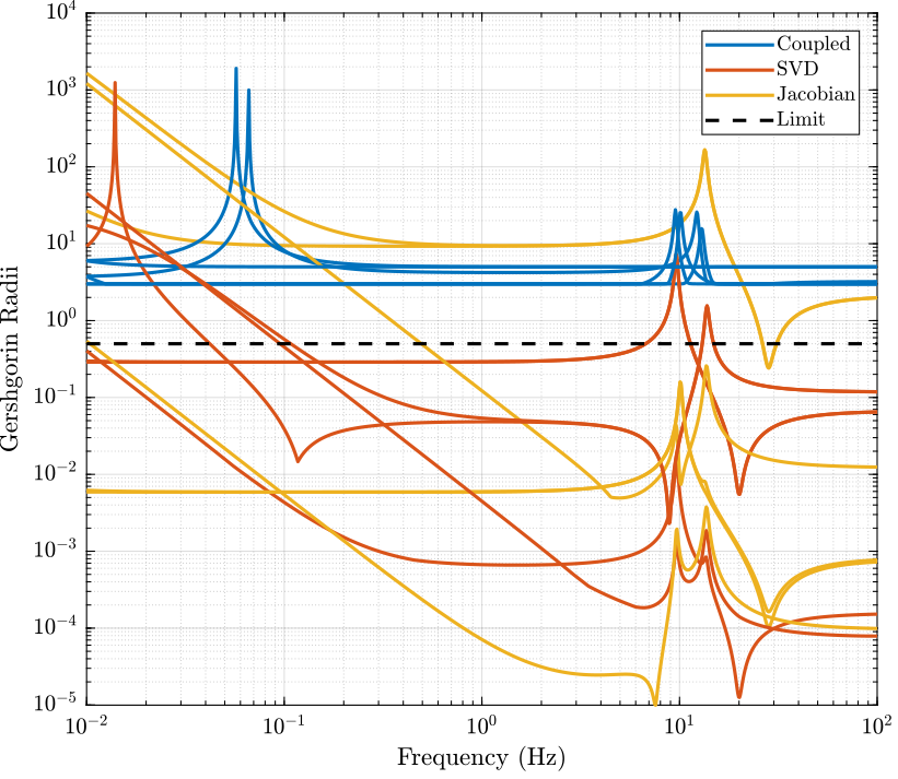
Figure 6: Gershgorin Radii of the Coupled and Decoupled plants

2.7 Decoupled Plant

Let’s see the bode plot of the decoupled plant \(G_d(s)\). \[ G_d(s) = U^T G_c(s) V \]

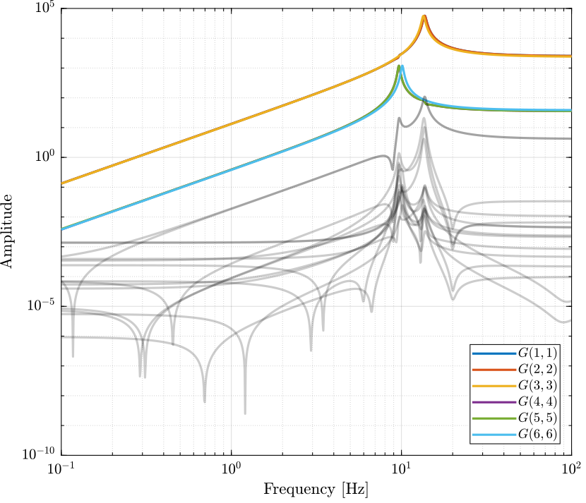
Figure 7: Decoupled Plant using SVD

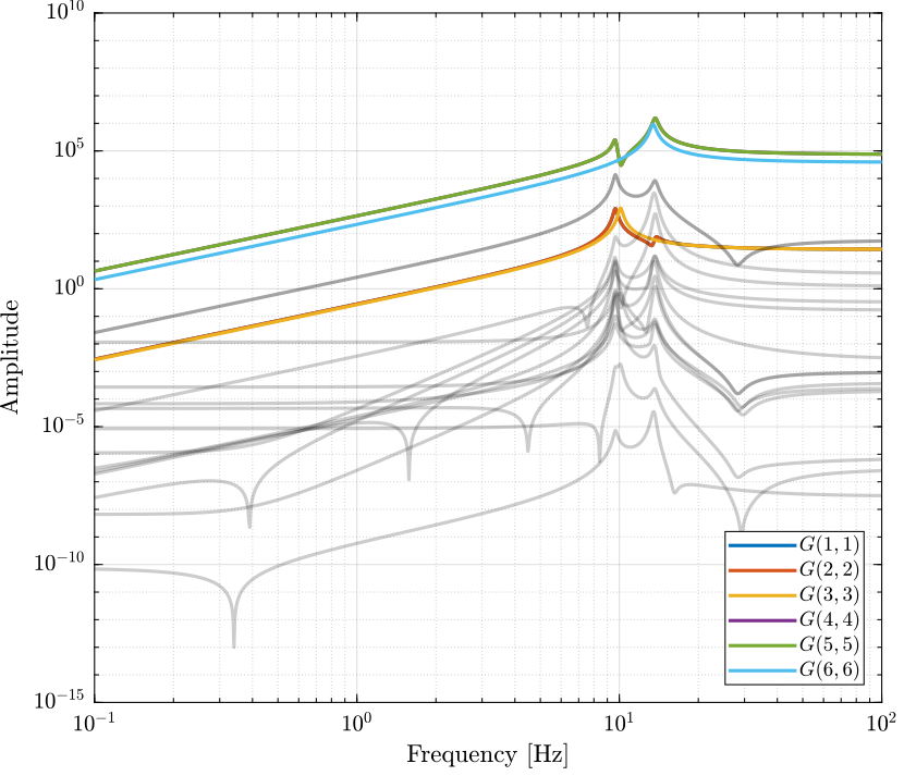
Figure 8: Decoupled Plant using the Jacobian

2.8 Diagonal Controller

The controller \(K\) is a diagonal controller consisting a low pass filters with a crossover frequency \(\omega_c\) and a DC gain \(C_g\).

wc = 2*pi*0.1; % Crossover Frequency [rad/s]
C_g = 50; % DC Gain

K = eye(6)*C_g/(s+wc);

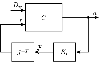
2.9 Centralized Control

The control diagram for the centralized control is shown below.

The controller \(K_c\) is “working” in an cartesian frame. The Jacobian is used to convert forces in the cartesian frame to forces applied by the actuators.

G_cen = feedback(G, inv(J')*K, [7:12], [1:6]);

2.10 SVD Control

The SVD control architecture is shown below. The matrices \(U\) and \(V\) are used to decoupled the plant \(G\).

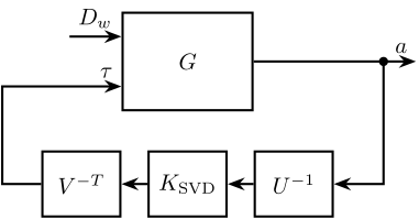
SVD Control

G_svd = feedback(G, pinv(V')*K*pinv(U), [7:12], [1:6]);

2.11 Results

Let’s first verify the stability of the closed-loop systems:

isstable(G_cen)

ans =
  logical
   1

isstable(G_svd)

ans =
  logical
   1

The obtained transmissibility in Open-loop, for the centralized control as well as for the SVD control are shown in Figure 11.

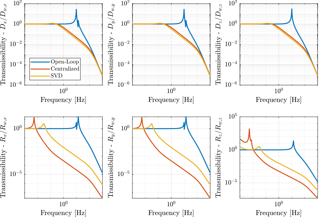
Figure 11: Obtained Transmissibility

3 Stewart Platform - Analytical Model

3.1 Characteristics

L  = 0.055;
Zc = 0;
m  = 0.2;
k  = 1e3;
c  = 2*0.1*sqrt(k*m);

Rx = 0.04;
Rz = 0.04;
Ix = m*Rx^2;
Iy = m*Rx^2;
Iz = m*Rz^2;

3.2 Mass Matrix

M = m*[1 0 0 0 Zc 0;
       0 1 0 -Zc 0 0;
       0 0 1 0 0 0;
       0 -Zc 0 Rx^2+Zc^2 0 0;
       Zc 0 0 0 Rx^2+Zc^2 0;
       0 0 0 0 0 Rz^2];

3.3 Jacobian Matrix

Bj=1/sqrt(6)*[ 1 1 -2 1 1 -2;
               sqrt(3) -sqrt(3) 0 sqrt(3) -sqrt(3) 0;
               sqrt(2) sqrt(2) sqrt(2) sqrt(2) sqrt(2) sqrt(2);
               0 0 L L -L -L;
               -L*2/sqrt(3) -L*2/sqrt(3) L/sqrt(3) L/sqrt(3) L/sqrt(3) L/sqrt(3);
               L*sqrt(2) -L*sqrt(2) L*sqrt(2) -L*sqrt(2) L*sqrt(2) -L*sqrt(2)];

3.4 Stifnness matrix and Damping matrix

kv = k/3; % [N/m]
kh = 0.5*k/3; % [N/m]

K = diag([3*kh,3*kh,3*kv,3*kv*Rx^2/2,3*kv*Rx^2/2,3*kh*Rx^2]); % Stiffness Matrix

C = c*K/100000; % Damping Matrix

3.5 State Space System

A  = [zeros(6) eye(6); -M\K -M\C];
Bw = [zeros(6); -eye(6)];
Bu = [zeros(6); M\Bj];
Co = [-M\K -M\C];
D  = [zeros(6) M\Bj];

ST = ss(A,[Bw Bu],Co,D);

OUT 1-6: 6 dof
IN 1-6 : ground displacement in the directions of the legs
IN 7-12: forces in the actuators.

ST.StateName = {'x';'y';'z';'theta_x';'theta_y';'theta_z';...
                'dx';'dy';'dz';'dtheta_x';'dtheta_y';'dtheta_z'};
ST.InputName = {'w1';'w2';'w3';'w4';'w5';'w6';...
                'u1';'u2';'u3';'u4';'u5';'u6'};
ST.OutputName = {'ax';'ay';'az';'atheta_x';'atheta_y';'atheta_z'};

3.6 Transmissibility

TR=ST*[eye(6); zeros(6)];

figure
subplot(231)
bodemag(TR(1,1),opts);
subplot(232)
bodemag(TR(2,2),opts);
subplot(233)
bodemag(TR(3,3),opts);
subplot(234)
bodemag(TR(4,4),opts);
subplot(235)
bodemag(TR(5,5),opts);
subplot(236)
bodemag(TR(6,6),opts);

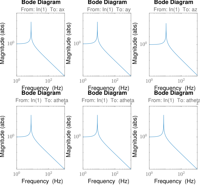
Figure 12: Transmissibility

3.7 Real approximation of \(G(j\omega)\) at decoupling frequency

sys1 = ST*[zeros(6); eye(6)]; % take only the forces inputs

dec_fr = 20;
H1 = evalfr(sys1,j*2*pi*dec_fr);
H2 = H1;
D = pinv(real(H2'*H2));
H1 = inv(D*real(H2'*diag(exp(j*angle(diag(H2*D*H2.'))/2)))) ;
[U,S,V] = svd(H1);

wf = logspace(-1,2,1000);
for i  = 1:length(wf)
    H = abs(evalfr(sys1,j*2*pi*wf(i)));
    H_dec = abs(evalfr(U'*sys1*V,j*2*pi*wf(i)));
    for j = 1:size(H,2)
        g_r1(i,j) =  (sum(H(j,:))-H(j,j))/H(j,j);
        g_r2(i,j) =  (sum(H_dec(j,:))-H_dec(j,j))/H_dec(j,j);
        %     keyboard
    end
    g_lim(i) = 0.5;
end

3.8 Coupled and Decoupled Plant “Gershgorin Radii”

figure;
title('Coupled plant')
loglog(wf,g_r1(:,1),wf,g_r1(:,2),wf,g_r1(:,3),wf,g_r1(:,4),wf,g_r1(:,5),wf,g_r1(:,6),wf,g_lim,'--');
legend('$a_x$','$a_y$','$a_z$','$\theta_x$','$\theta_y$','$\theta_z$','Limit');
xlabel('Frequency (Hz)'); ylabel('Gershgorin Radii')

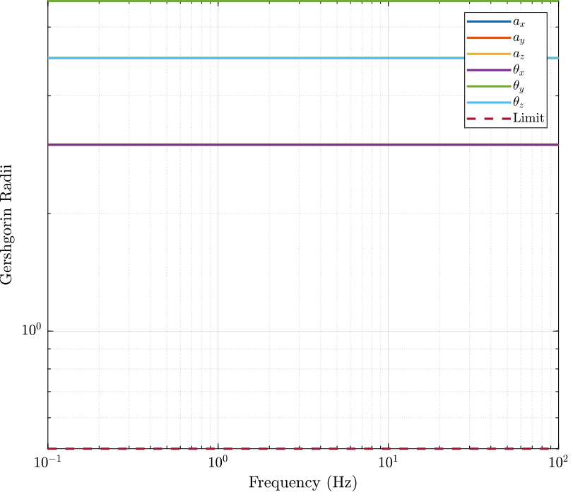
Figure 13: Gershorin Raddi for the coupled plant

figure;
title('Decoupled plant (10 Hz)')
loglog(wf,g_r2(:,1),wf,g_r2(:,2),wf,g_r2(:,3),wf,g_r2(:,4),wf,g_r2(:,5),wf,g_r2(:,6),wf,g_lim,'--');
legend('$S_1$','$S_2$','$S_3$','$S_4$','$S_5$','$S_6$','Limit');
xlabel('Frequency (Hz)'); ylabel('Gershgorin Radii')

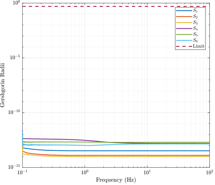
Figure 14: Gershorin Raddi for the decoupled plant

3.9 Decoupled Plant

figure;
bodemag(U'*sys1*V,opts)

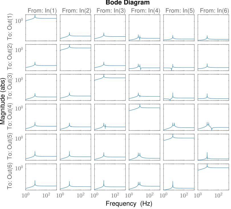
Figure 15: Decoupled Plant

3.10 Controller

fc = 2*pi*0.1; % Crossover Frequency [rad/s]
c_gain = 50; %

cont = eye(6)*c_gain/(s+fc);

3.11 Closed Loop System

FEEDIN  = [7:12]; % Input of controller
FEEDOUT = [1:6]; % Output of controller

Centralized Control

STcen = feedback(ST, inv(Bj)*cont, FEEDIN, FEEDOUT);
TRcen = STcen*[eye(6); zeros(6)];

SVD Control

STsvd = feedback(ST, pinv(V')*cont*pinv(U), FEEDIN, FEEDOUT);
TRsvd = STsvd*[eye(6); zeros(6)];

3.12 Results

figure
subplot(231)
bodemag(TR(1,1),TRcen(1,1),TRsvd(1,1),opts)
legend('OL','Centralized','SVD')
subplot(232)
bodemag(TR(2,2),TRcen(2,2),TRsvd(2,2),opts)
legend('OL','Centralized','SVD')
subplot(233)
bodemag(TR(3,3),TRcen(3,3),TRsvd(3,3),opts)
legend('OL','Centralized','SVD')
subplot(234)
bodemag(TR(4,4),TRcen(4,4),TRsvd(4,4),opts)
legend('OL','Centralized','SVD')
subplot(235)
bodemag(TR(5,5),TRcen(5,5),TRsvd(5,5),opts)
legend('OL','Centralized','SVD')
subplot(236)
bodemag(TR(6,6),TRcen(6,6),TRsvd(6,6),opts)
legend('OL','Centralized','SVD')

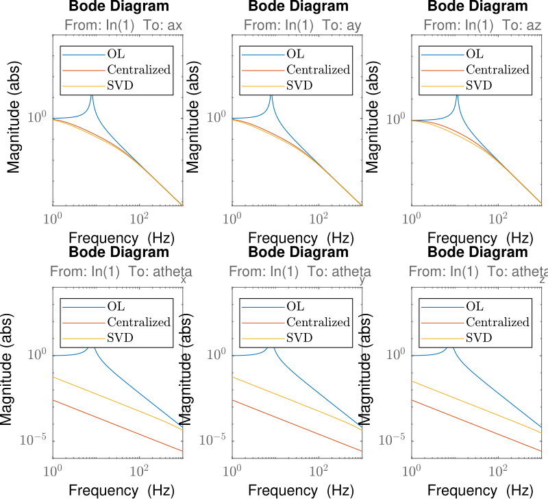
Figure 16: Comparison of the obtained transmissibility for the centralized control and the SVD control

SVD Control

Table of Contents

1 Gravimeter - Simscape Model

1.1 Simulink

2 Stewart Platform - Simscape Model

2.1 Jacobian

2.2 Simscape Model

2.3 Identification of the plant

2.4 Obtained Dynamics

2.5 Real Approximation of \(G\) at the decoupling frequency

2.6 Verification of the decoupling using the “Gershgorin Radii”

2.7 Decoupled Plant

2.8 Diagonal Controller

2.9 Centralized Control

2.10 SVD Control

2.11 Results

3 Stewart Platform - Analytical Model

3.1 Characteristics

3.2 Mass Matrix

3.3 Jacobian Matrix

3.4 Stifnness matrix and Damping matrix

3.5 State Space System

3.6 Transmissibility

3.7 Real approximation of \(G(j\omega)\) at decoupling frequency

3.8 Coupled and Decoupled Plant “Gershgorin Radii”

3.9 Decoupled Plant

3.10 Controller

3.11 Closed Loop System

3.12 Results