Stewart Platform - Decentralized Active Damping

1. Inertial Control
2. Integral Force Feedback
3. Direct Velocity Feedback
4. Compliance and Transmissibility Comparison

The following decentralized active damping techniques are briefly studied:

Inertial Control (proportional feedback of the absolute velocity): Section 1
Integral Force Feedback: Section 2
Direct feedback of the relative velocity of each strut: Section 3

1 Inertial Control

The Matlab script corresponding to this section is accessible here.

To run the script, open the Simulink Project, and type run active_damping_inertial.m.

1.1 Identification of the Dynamics

stewart = initializeStewartPlatform();
stewart = initializeFramesPositions(stewart, 'H', 90e-3, 'MO_B', 45e-3);
stewart = generateGeneralConfiguration(stewart);
stewart = computeJointsPose(stewart);
stewart = initializeStrutDynamics(stewart);
stewart = initializeJointDynamics(stewart, 'type_F', 'universal_p', 'type_M', 'spherical_p');
stewart = initializeCylindricalPlatforms(stewart);
stewart = initializeCylindricalStruts(stewart);
stewart = computeJacobian(stewart);
stewart = initializeStewartPose(stewart);
stewart = initializeInertialSensor(stewart, 'type', 'accelerometer', 'freq', 5e3);

ground = initializeGround('type', 'rigid', 'rot_point', stewart.platform_F.FO_A);
payload = initializePayload('type', 'none');

%% Options for Linearized
options = linearizeOptions;
options.SampleTime = 0;

%% Name of the Simulink File
mdl = 'stewart_platform_model';

%% Input/Output definition
clear io; io_i = 1;
io(io_i) = linio([mdl, '/Controller'],        1, 'openinput');  io_i = io_i + 1; % Actuator Force Inputs [N]
io(io_i) = linio([mdl, '/Stewart Platform'],  1, 'openoutput', [], 'Vm'); io_i = io_i + 1; % Absolute velocity of each leg [m/s]

%% Run the linearization
G = linearize(mdl, io, options);
G.InputName  = {'F1', 'F2', 'F3', 'F4', 'F5', 'F6'};
G.OutputName = {'Vm1', 'Vm2', 'Vm3', 'Vm4', 'Vm5', 'Vm6'};

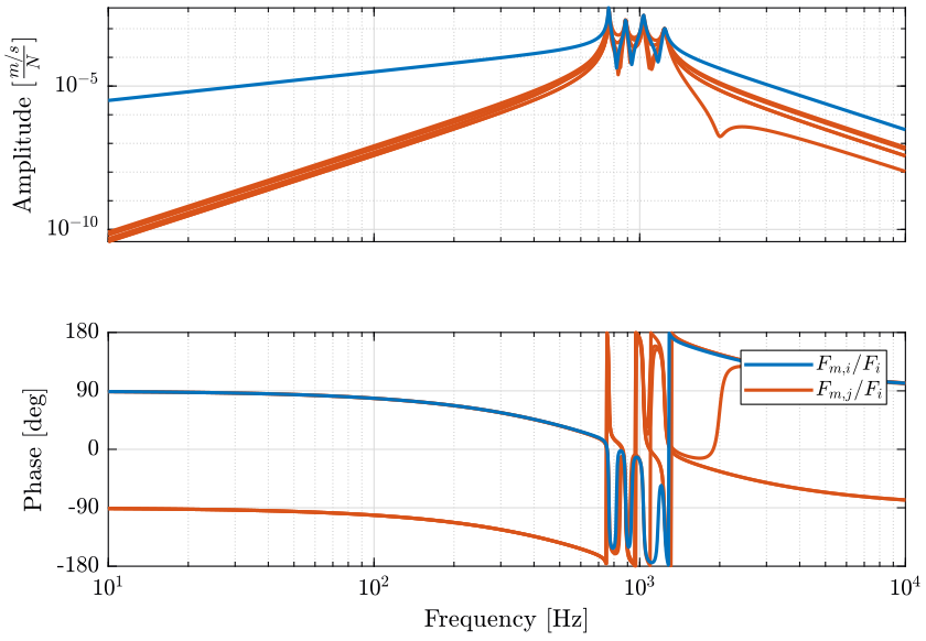
The transfer function from actuator forces to force sensors is shown in Figure 1.

Figure 1: Transfer function from the Actuator force \(F_{i}\) to the absolute velocity of the same leg \(v_{m,i}\) and to the absolute velocity of the other legs \(v_{m,j}\) with \(i \neq j\) in grey (png, pdf)

1.2 Effect of the Flexible Joint stiffness and Actuator amplification on the Dynamics

We add some stiffness and damping in the flexible joints and we re-identify the dynamics.

stewart = initializeJointDynamics(stewart, 'type_F', 'universal', 'type_M', 'spherical');
Gf = linearize(mdl, io, options);
Gf.InputName  = {'F1', 'F2', 'F3', 'F4', 'F5', 'F6'};
Gf.OutputName = {'Vm1', 'Vm2', 'Vm3', 'Vm4', 'Vm5', 'Vm6'};

We now use the amplified actuators and re-identify the dynamics

stewart = initializeAmplifiedStrutDynamics(stewart);
Ga = linearize(mdl, io, options);
Ga.InputName  = {'F1', 'F2', 'F3', 'F4', 'F5', 'F6'};
Ga.OutputName = {'Vm1', 'Vm2', 'Vm3', 'Vm4', 'Vm5', 'Vm6'};

The new dynamics from force actuator to force sensor is shown in Figure 2.

Figure 2: Transfer function from the Actuator force \(F_{i}\) to the absolute velocity sensor \(v_{m,i}\) (png, pdf)

1.3 Obtained Damping

The control is a performed in a decentralized manner. The \(6 \times 6\) control is a diagonal matrix with pure proportional action on the diagonal: \[ K(s) = g \begin{bmatrix} 1 & & 0 \\ & \ddots & \\ 0 & & 1 \end{bmatrix} \]

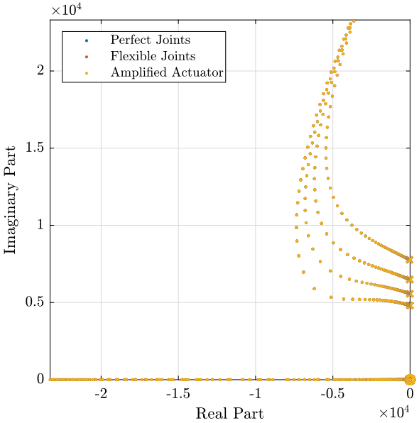
The root locus is shown in figure 3.

Figure 3: Root Locus plot with Decentralized Inertial Control when considering the stiffness of flexible joints (png, pdf)

1.4 Conclusion

We do not have guaranteed stability with Inertial control. This is because of the flexibility inside the internal sensor.

2 Integral Force Feedback

The Matlab script corresponding to this section is accessible here.

To run the script, open the Simulink Project, and type run active_damping_iff.m.

2.1 Identification of the Dynamics with perfect Joints

We first initialize the Stewart platform without joint stiffness.

stewart = initializeStewartPlatform();
stewart = initializeFramesPositions(stewart, 'H', 90e-3, 'MO_B', 45e-3);
stewart = generateGeneralConfiguration(stewart);
stewart = computeJointsPose(stewart);
stewart = initializeStrutDynamics(stewart);
stewart = initializeJointDynamics(stewart, 'type_F', 'universal_p', 'type_M', 'spherical_p');
stewart = initializeCylindricalPlatforms(stewart);
stewart = initializeCylindricalStruts(stewart);
stewart = computeJacobian(stewart);
stewart = initializeStewartPose(stewart);
stewart = initializeInertialSensor(stewart, 'type', 'none');

ground = initializeGround('type', 'rigid', 'rot_point', stewart.platform_F.FO_A);
payload = initializePayload('type', 'none');

controller = initializeController('type', 'open-loop');

And we identify the dynamics from force actuators to force sensors.

%% Options for Linearized
options = linearizeOptions;
options.SampleTime = 0;

%% Name of the Simulink File
mdl = 'stewart_platform_model';

%% Input/Output definition
clear io; io_i = 1;
io(io_i) = linio([mdl, '/Controller'],        1, 'openinput');  io_i = io_i + 1; % Actuator Force Inputs [N]
io(io_i) = linio([mdl, '/Stewart Platform'],  1, 'openoutput', [], 'Taum'); io_i = io_i + 1; % Force Sensor Outputs [N]

%% Run the linearization
G = linearize(mdl, io, options);
G.InputName  = {'F1', 'F2', 'F3', 'F4', 'F5', 'F6'};
G.OutputName = {'Fm1', 'Fm2', 'Fm3', 'Fm4', 'Fm5', 'Fm6'};

The transfer function from actuator forces to force sensors is shown in Figure 4.

Figure 4: Transfer function from the Actuator force \(F_{i}\) to the Force sensor of the same leg \(F_{m,i}\) and to the force sensor of the other legs \(F_{m,j}\) with \(i \neq j\) in grey (png, pdf)

2.2 Effect of the Flexible Joint stiffness and Actuator amplification on the Dynamics

We add some stiffness and damping in the flexible joints and we re-identify the dynamics.

stewart = initializeJointDynamics(stewart, 'type_F', 'universal', 'type_M', 'spherical');
Gf = linearize(mdl, io, options);
Gf.InputName  = {'F1', 'F2', 'F3', 'F4', 'F5', 'F6'};
Gf.OutputName = {'Fm1', 'Fm2', 'Fm3', 'Fm4', 'Fm5', 'Fm6'};

We now use the amplified actuators and re-identify the dynamics

stewart = initializeAmplifiedStrutDynamics(stewart);
Ga = linearize(mdl, io, options);
Ga.InputName  = {'F1', 'F2', 'F3', 'F4', 'F5', 'F6'};
Ga.OutputName = {'Fm1', 'Fm2', 'Fm3', 'Fm4', 'Fm5', 'Fm6'};

The new dynamics from force actuator to force sensor is shown in Figure 5.

Figure 5: Transfer function from the Actuator force \(F_{i}\) to the force sensor \(F_{m,i}\) (png, pdf)

2.3 Obtained Damping

The control is a performed in a decentralized manner. The \(6 \times 6\) control is a diagonal matrix with pure integration action on the diagonal: \[ K(s) = g \begin{bmatrix} \frac{1}{s} & & 0 \\ & \ddots & \\ 0 & & \frac{1}{s} \end{bmatrix} \]

The root locus is shown in figure 6 and the obtained pole damping function of the control gain is shown in figure 7.

Figure 6: Root Locus plot with Decentralized Integral Force Feedback when considering the stiffness of flexible joints (png, pdf)

Figure 7: Damping of the poles with respect to the gain of the Decentralized Integral Force Feedback when considering the stiffness of flexible joints (png, pdf)

2.4 Conclusion

The joint stiffness has a huge impact on the attainable active damping performance when using force sensors. Thus, if Integral Force Feedback is to be used in a Stewart platform with flexible joints, the rotational stiffness of the joints should be minimized.

3 Direct Velocity Feedback

The Matlab script corresponding to this section is accessible here.

To run the script, open the Simulink Project, and type run active_damping_dvf.m.

3.1 Identification of the Dynamics with perfect Joints

We first initialize the Stewart platform without joint stiffness.

stewart = initializeStewartPlatform();
stewart = initializeFramesPositions(stewart, 'H', 90e-3, 'MO_B', 45e-3);
stewart = generateGeneralConfiguration(stewart);
stewart = computeJointsPose(stewart);
stewart = initializeStrutDynamics(stewart);
stewart = initializeJointDynamics(stewart, 'type_F', 'universal_p', 'type_M', 'spherical_p');
stewart = initializeCylindricalPlatforms(stewart);
stewart = initializeCylindricalStruts(stewart);
stewart = computeJacobian(stewart);
stewart = initializeStewartPose(stewart);
stewart = initializeInertialSensor(stewart, 'type', 'none');

ground = initializeGround('type', 'rigid', 'rot_point', stewart.platform_F.FO_A);
payload = initializePayload('type', 'none');

And we identify the dynamics from force actuators to force sensors.

%% Options for Linearized
options = linearizeOptions;
options.SampleTime = 0;

%% Name of the Simulink File
mdl = 'stewart_platform_model';

%% Input/Output definition
clear io; io_i = 1;
io(io_i) = linio([mdl, '/Controller'],        1, 'openinput');  io_i = io_i + 1; % Actuator Force Inputs [N]
io(io_i) = linio([mdl, '/Stewart Platform'],  1, 'openoutput', [], 'dLm'); io_i = io_i + 1; % Relative Displacement Outputs [m]

%% Run the linearization
G = linearize(mdl, io, options);
G.InputName  = {'F1', 'F2', 'F3', 'F4', 'F5', 'F6'};
G.OutputName = {'Dm1', 'Dm2', 'Dm3', 'Dm4', 'Dm5', 'Dm6'};

The transfer function from actuator forces to relative motion sensors is shown in Figure 8.

Figure 8: Transfer function from the Actuator force \(F_{i}\) to the Relative Motion Sensor \(D_{m,j}\) with \(i \neq j\) (png, pdf)

3.2 Effect of the Flexible Joint stiffness and Actuator amplification on the Dynamics

We add some stiffness and damping in the flexible joints and we re-identify the dynamics.

stewart = initializeJointDynamics(stewart, 'type_F', 'universal', 'type_M', 'spherical');
Gf = linearize(mdl, io, options);
Gf.InputName  = {'F1', 'F2', 'F3', 'F4', 'F5', 'F6'};
Gf.OutputName = {'Dm1', 'Dm2', 'Dm3', 'Dm4', 'Dm5', 'Dm6'};

We now use the amplified actuators and re-identify the dynamics

stewart = initializeAmplifiedStrutDynamics(stewart);
Ga = linearize(mdl, io, options);
Ga.InputName  = {'F1', 'F2', 'F3', 'F4', 'F5', 'F6'};
Ga.OutputName = {'Dm1', 'Dm2', 'Dm3', 'Dm4', 'Dm5', 'Dm6'};

The new dynamics from force actuator to relative motion sensor is shown in Figure 9.

Figure 9: Transfer function from the Actuator force \(F_{i}\) to the relative displacement sensor \(D_{m,i}\) (png, pdf)

3.3 Obtained Damping

The control is a performed in a decentralized manner. The \(6 \times 6\) control is a diagonal matrix with pure derivative action on the diagonal: \[ K(s) = g \begin{bmatrix} s & & \\ & \ddots & \\ & & s \end{bmatrix} \]

The root locus is shown in figure 10.

Figure 10: Root Locus plot with Direct Velocity Feedback when considering the Stiffness of flexible joints (png, pdf)

3.4 Conclusion

Joint stiffness does increase the resonance frequencies of the system but does not change the attainable damping when using relative motion sensors.

4 Compliance and Transmissibility Comparison

4.1 Initialization

We first initialize the Stewart platform without joint stiffness.

stewart = initializeStewartPlatform();
stewart = initializeFramesPositions(stewart, 'H', 90e-3, 'MO_B', 45e-3);
stewart = generateGeneralConfiguration(stewart);
stewart = computeJointsPose(stewart);
stewart = initializeStrutDynamics(stewart);
stewart = initializeJointDynamics(stewart, 'type_F', 'universal_p', 'type_M', 'spherical_p');
stewart = initializeCylindricalPlatforms(stewart);
stewart = initializeCylindricalStruts(stewart);
stewart = computeJacobian(stewart);
stewart = initializeStewartPose(stewart);
stewart = initializeInertialSensor(stewart, 'type', 'none');

The rotation point of the ground is located at the origin of frame \(\{A\}\).

ground = initializeGround('type', 'rigid', 'rot_point', stewart.platform_F.FO_A);
payload = initializePayload('type', 'none');

4.2 Identification

Let’s first identify the transmissibility and compliance in the open-loop case.

controller = initializeController('type', 'open-loop');
[T_ol, T_norm_ol, freqs] = computeTransmissibility();
[C_ol, C_norm_ol, freqs] = computeCompliance();

Now, let’s identify the transmissibility and compliance for the Integral Force Feedback architecture.

controller = initializeController('type', 'iff');
G_iff = (2e4/s)*eye(6);

[T_iff, T_norm_iff, ~] = computeTransmissibility();
[C_iff, C_norm_iff, ~] = computeCompliance();

And for the Direct Velocity Feedback.

controller = initializeController('type', 'dvf');
G_dvf = 1e4*s/(1+s/2/pi/5000)*eye(6);

[T_dvf, T_norm_dvf, ~] = computeTransmissibility();
[C_dvf, C_norm_dvf, ~] = computeCompliance();

4.3 Results

Figure 11: Obtained transmissibility for Open-Loop Control (Blue), Integral Force Feedback (Red) and Direct Velocity Feedback (Yellow) (png, pdf)

Figure 12: Obtained compliance for Open-Loop Control (Blue), Integral Force Feedback (Red) and Direct Velocity Feedback (Yellow) (png, pdf)

Figure 13: Frobenius norm of the Transmissibility and Compliance Matrices (png, pdf)

Stewart Platform - Decentralized Active Damping

Table of Contents

1 Inertial Control

1.1 Identification of the Dynamics

1.2 Effect of the Flexible Joint stiffness and Actuator amplification on the Dynamics

1.3 Obtained Damping

1.4 Conclusion

2 Integral Force Feedback

2.1 Identification of the Dynamics with perfect Joints

2.2 Effect of the Flexible Joint stiffness and Actuator amplification on the Dynamics

2.3 Obtained Damping

2.4 Conclusion

3 Direct Velocity Feedback

3.1 Identification of the Dynamics with perfect Joints

3.2 Effect of the Flexible Joint stiffness and Actuator amplification on the Dynamics

3.3 Obtained Damping

3.4 Conclusion

4 Compliance and Transmissibility Comparison

4.1 Initialization

4.2 Identification

4.3 Results