Cubic configuration for the Stewart Platform
Table of Contents
- 1. Questions we wish to answer with this analysis
- 2. Configuration Analysis - Stiffness Matrix
- 2.1. Cubic Stewart platform centered with the cube center - Jacobian estimated at the cube center
- 2.2. Cubic Stewart platform centered with the cube center - Jacobian not estimated at the cube center
- 2.3. Cubic Stewart platform not centered with the cube center - Jacobian estimated at the cube center
- 2.4. Cubic Stewart platform not centered with the cube center - Jacobian estimated at the Stewart platform center
- 2.5. Conclusion
- 3. Cubic size analysis
- 4. initializeCubicConfiguration
- 5. Tests
The discovery of the Cubic configuration is done in geng94_six_degree_of_freed_activ. Further analysis is conducted in jafari03_orthog_gough_stewar_platf_microm.
People using orthogonal/cubic configuration: preumont07_six_axis_singl_stage_activ.
The specificity of the Cubic configuration is that each actuator is orthogonal with the others.
To generate and study the Cubic configuration, initializeCubicConfiguration is used (description in section 4).
According to preumont07_six_axis_singl_stage_activ, the cubic configuration provides a uniform stiffness in all directions and minimizes the crosscoupling from actuator to sensor of different legs (being orthogonal to each other).
1 Questions we wish to answer with this analysis
The goal is to study the benefits of using a cubic configuration:
- Equal stiffness in all the degrees of freedom?
- No coupling between the actuators?
- Is the center of the cube an important point?
2 Configuration Analysis - Stiffness Matrix
2.1 Cubic Stewart platform centered with the cube center - Jacobian estimated at the cube center
We create a cubic Stewart platform (figure 1) in such a way that the center of the cube (black dot) is located at the center of the Stewart platform (blue dot). The Jacobian matrix is estimated at the location of the center of the cube.
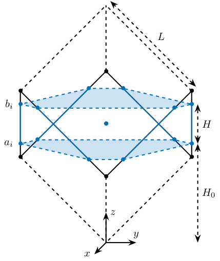
Figure 1: Centered cubic configuration
opts = struct(...
    'H_tot', 100, ... % Total height of the Hexapod [mm]
    'L',     200/sqrt(3), ... % Size of the Cube [mm]
    'H',     60, ... % Height between base joints and platform joints [mm]
    'H0',    200/2-60/2 ... % Height between the corner of the cube and the plane containing the base joints [mm]
    );
stewart = initializeCubicConfiguration(opts);
opts = struct(...
    'Jd_pos', [0, 0, -50], ... % Position of the Jacobian for displacement estimation from the top of the mobile platform [mm]
    'Jf_pos', [0, 0, -50]  ... % Position of the Jacobian for force location from the top of the mobile platform [mm]
    );
stewart = computeGeometricalProperties(stewart, opts);

save('./mat/stewart.mat', 'stewart');
K = stewart.Jf'*stewart.Jf;
| 2 | 1.9e-18 | -2.3e-17 | 1.8e-18 | 5.5e-17 | -1.5e-17 |
| 1.9e-18 | 2 | 6.8e-18 | -6.1e-17 | -1.6e-18 | 4.8e-18 |
| -2.3e-17 | 6.8e-18 | 2 | -6.7e-18 | 4.9e-18 | 5.3e-19 |
| 1.8e-18 | -6.1e-17 | -6.7e-18 | 0.0067 | -2.3e-20 | -6.1e-20 |
| 5.5e-17 | -1.6e-18 | 4.9e-18 | -2.3e-20 | 0.0067 | 1e-18 |
| -1.5e-17 | 4.8e-18 | 5.3e-19 | -6.1e-20 | 1e-18 | 0.027 |
2.2 Cubic Stewart platform centered with the cube center - Jacobian not estimated at the cube center
We create a cubic Stewart platform with center of the cube located at the center of the Stewart platform (figure 1). The Jacobian matrix is not estimated at the location of the center of the cube.
opts = struct(...
    'H_tot', 100, ... % Total height of the Hexapod [mm]
    'L',     200/sqrt(3), ... % Size of the Cube [mm]
    'H',     60, ... % Height between base joints and platform joints [mm]
    'H0',    200/2-60/2 ... % Height between the corner of the cube and the plane containing the base joints [mm]
    );
stewart = initializeCubicConfiguration(opts);
opts = struct(...
    'Jd_pos', [0, 0, 0], ... % Position of the Jacobian for displacement estimation from the top of the mobile platform [mm]
    'Jf_pos', [0, 0, 0]  ... % Position of the Jacobian for force location from the top of the mobile platform [mm]
    );
stewart = computeGeometricalProperties(stewart, opts);
K = stewart.Jf'*stewart.Jf;
| 2 | 1.9e-18 | -2.3e-17 | 1.5e-18 | -0.1 | -1.5e-17 |
| 1.9e-18 | 2 | 6.8e-18 | 0.1 | -1.6e-18 | 4.8e-18 |
| -2.3e-17 | 6.8e-18 | 2 | -5.1e-19 | -5.5e-18 | 5.3e-19 |
| 1.5e-18 | 0.1 | -5.1e-19 | 0.012 | -3e-19 | 3.1e-19 |
| -0.1 | -1.6e-18 | -5.5e-18 | -3e-19 | 0.012 | 1.9e-18 |
| -1.5e-17 | 4.8e-18 | 5.3e-19 | 3.1e-19 | 1.9e-18 | 0.027 |
2.3 Cubic Stewart platform not centered with the cube center - Jacobian estimated at the cube center
Here, the "center" of the Stewart platform is not at the cube center (figure 2). The Jacobian is estimated at the cube center.
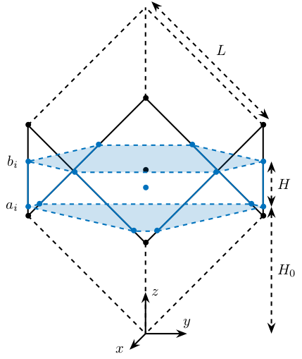
Figure 2: Not centered cubic configuration
The center of the cube is at \(z = 110\). The Stewart platform is from \(z = H_0 = 75\) to \(z = H_0 + H_{tot} = 175\). The center height of the Stewart platform is then at \(z = \frac{175-75}{2} = 50\). The center of the cube from the top platform is at \(z = 110 - 175 = -65\).
opts = struct(...
    'H_tot', 100,         ... % Total height of the Hexapod [mm]
    'L',     220/sqrt(3), ... % Size of the Cube [mm]
    'H',     60,          ... % Height between base joints and platform joints [mm]
    'H0',    75           ... % Height between the corner of the cube and the plane containing the base joints [mm]
    );
stewart = initializeCubicConfiguration(opts);
opts = struct(...
    'Jd_pos', [0, 0, -65], ... % Position of the Jacobian for displacement estimation from the top of the mobile platform [mm]
    'Jf_pos', [0, 0, -65]  ... % Position of the Jacobian for force location from the top of the mobile platform [mm]
    );
stewart = computeGeometricalProperties(stewart, opts);
K = stewart.Jf'*stewart.Jf;
| 2 | -1.8e-17 | 2.6e-17 | 3.3e-18 | 0.04 | 1.7e-19 |
| -1.8e-17 | 2 | 1.9e-16 | -0.04 | 2.2e-19 | -5.3e-19 |
| 2.6e-17 | 1.9e-16 | 2 | -8.9e-18 | 6.5e-19 | -5.8e-19 |
| 3.3e-18 | -0.04 | -8.9e-18 | 0.0089 | -9.3e-20 | 9.8e-20 |
| 0.04 | 2.2e-19 | 6.5e-19 | -9.3e-20 | 0.0089 | -2.4e-18 |
| 1.7e-19 | -5.3e-19 | -5.8e-19 | 9.8e-20 | -2.4e-18 | 0.032 |
We obtain \(k_x = k_y = k_z\) and \(k_{\theta_x} = k_{\theta_y}\), but the Stiffness matrix is not diagonal.
2.4 Cubic Stewart platform not centered with the cube center - Jacobian estimated at the Stewart platform center
Here, the "center" of the Stewart platform is not at the cube center. The Jacobian is estimated at the center of the Stewart platform.
The center of the cube is at \(z = 110\). The Stewart platform is from \(z = H_0 = 75\) to \(z = H_0 + H_{tot} = 175\). The center height of the Stewart platform is then at \(z = \frac{175-75}{2} = 50\). The center of the cube from the top platform is at \(z = 110 - 175 = -65\).
opts = struct(...
    'H_tot', 100, ... % Total height of the Hexapod [mm]
    'L',     220/sqrt(3), ... % Size of the Cube [mm]
    'H',     60, ... % Height between base joints and platform joints [mm]
    'H0',    75 ... % Height between the corner of the cube and the plane containing the base joints [mm]
    );
stewart = initializeCubicConfiguration(opts);
opts = struct(...
    'Jd_pos', [0, 0, -60], ... % Position of the Jacobian for displacement estimation from the top of the mobile platform [mm]
    'Jf_pos', [0, 0, -60]  ... % Position of the Jacobian for force location from the top of the mobile platform [mm]
    );
stewart = computeGeometricalProperties(stewart, opts);
K = stewart.Jf'*stewart.Jf;
| 2 | -1.8e-17 | 2.6e-17 | -5.7e-19 | 0.03 | 1.7e-19 |
| -1.8e-17 | 2 | 1.9e-16 | -0.03 | 2.2e-19 | -5.3e-19 |
| 2.6e-17 | 1.9e-16 | 2 | -1.5e-17 | 6.5e-19 | -5.8e-19 |
| -5.7e-19 | -0.03 | -1.5e-17 | 0.0085 | 4.9e-20 | 1.7e-19 |
| 0.03 | 2.2e-19 | 6.5e-19 | 4.9e-20 | 0.0085 | -1.1e-18 |
| 1.7e-19 | -5.3e-19 | -5.8e-19 | 1.7e-19 | -1.1e-18 | 0.032 |
We obtain \(k_x = k_y = k_z\) and \(k_{\theta_x} = k_{\theta_y}\), but the Stiffness matrix is not diagonal.
2.5 Conclusion
- The cubic configuration permits to have \(k_x = k_y = k_z\) and \(k_{\theta\x} = k_{\theta_y}\)
- The stiffness matrix \(K\) is diagonal for the cubic configuration if the Stewart platform and the cube are centered and the Jacobian is estimated at the cube center
3 Cubic size analysis
We here study the effect of the size of the cube used for the Stewart configuration.
We fix the height of the Stewart platform, the center of the cube is at the center of the Stewart platform.
We only vary the size of the cube.
H_cubes = 250:20:350;
stewarts = {zeros(length(H_cubes), 1)};
for i = 1:length(H_cubes)
  H_cube = H_cubes(i);
  H_tot = 100;
  H = 80;

  opts = struct(...
      'H_tot', H_tot, ... % Total height of the Hexapod [mm]
      'L',     H_cube/sqrt(3), ... % Size of the Cube [mm]
      'H',     H, ... % Height between base joints and platform joints [mm]
      'H0',    H_cube/2-H/2 ... % Height between the corner of the cube and the plane containing the base joints [mm]
      );
  stewart = initializeCubicConfiguration(opts);

  opts = struct(...
      'Jd_pos', [0, 0, H_cube/2-opts.H0-opts.H_tot], ... % Position of the Jacobian for displacement estimation from the top of the mobile platform [mm]
      'Jf_pos', [0, 0, H_cube/2-opts.H0-opts.H_tot]  ... % Position of the Jacobian for force location from the top of the mobile platform [mm]
      );
  stewart = computeGeometricalProperties(stewart, opts);
  stewarts(i) = {stewart};
end
The Stiffness matrix is computed for all generated Stewart platforms.
Ks = zeros(6, 6, length(H_cube));
for i = 1:length(H_cubes)
  Ks(:, :, i) = stewarts{i}.Jd'*stewarts{i}.Jd;
end
The only elements of \(K\) that vary are \(k_{\theta_x} = k_{\theta_y}\) and \(k_{\theta_z}\).
Finally, we plot \(k_{\theta_x} = k_{\theta_y}\) and \(k_{\theta_z}\)
figure;
hold on;
plot(H_cubes, squeeze(Ks(4, 4, :)), 'DisplayName', '$k_{\theta_x}$');
plot(H_cubes, squeeze(Ks(6, 6, :)), 'DisplayName', '$k_{\theta_z}$');
hold off;
legend('location', 'northwest');
xlabel('Cube Size [mm]'); ylabel('Rotational stiffnes [normalized]');
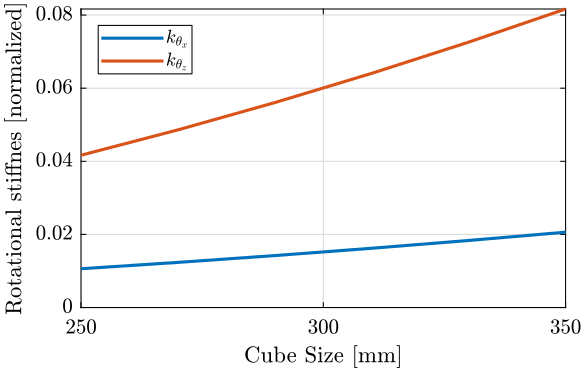
Figure 3: \(k_{\theta_x} = k_{\theta_y}\) and \(k_{\theta_z}\) function of the size of the cube
We observe that \(k_{\theta_x} = k_{\theta_y}\) and \(k_{\theta_z}\) increase linearly with the cube size.
In order to maximize the rotational stiffness of the Stewart platform, the size of the cube should be the highest possible. In that case, the legs will the further separated. Size of the cube is then limited by allowed space.
4 initializeCubicConfiguration
4.1 Function description
function [stewart] = initializeCubicConfiguration(opts_param)
4.2 Optional Parameters
Default values for opts.
opts = struct(...
    'H_tot', 90,  ... % Total height of the Hexapod [mm]
    'L',     110, ... % Size of the Cube [mm]
    'H',     40,  ... % Height between base joints and platform joints [mm]
    'H0',    75   ... % Height between the corner of the cube and the plane containing the base joints [mm]
    );
Populate opts with input parameters
if exist('opts_param','var')
    for opt = fieldnames(opts_param)'
        opts.(opt{1}) = opts_param.(opt{1});
    end
end
4.3 Cube Creation
points = [0, 0, 0; ...
          0, 0, 1; ...
          0, 1, 0; ...
          0, 1, 1; ...
          1, 0, 0; ...
          1, 0, 1; ...
          1, 1, 0; ...
          1, 1, 1];
points = opts.L*points;
We create the rotation matrix to rotate the cube
sx = cross([1, 1, 1], [1 0 0]);
sx = sx/norm(sx);

sy = -cross(sx, [1, 1, 1]);
sy = sy/norm(sy);

sz = [1, 1, 1];
sz = sz/norm(sz);

R = [sx', sy', sz']';
We use to rotation matrix to rotate the cube
cube = zeros(size(points));
for i = 1:size(points, 1)
  cube(i, :) = R * points(i, :)';
end
4.4 Vectors of each leg
leg_indices = [3, 4; ...
               2, 4; ...
               2, 6; ...
               5, 6; ...
               5, 7; ...
               3, 7];
Vectors are:
legs = zeros(6, 3);
legs_start = zeros(6, 3);

for i = 1:6
  legs(i, :) = cube(leg_indices(i, 2), :) - cube(leg_indices(i, 1), :);
  legs_start(i, :) = cube(leg_indices(i, 1), :);
end
4.5 Verification of Height of the Stewart Platform
If the Stewart platform is not contained in the cube, throw an error.
Hmax = cube(4, 3) - cube(2, 3);
if opts.H0 < cube(2, 3)
  error(sprintf('H0 is not high enought. Minimum H0 = %.1f', cube(2, 3)));
else if opts.H0 + opts.H > cube(4, 3)
  error(sprintf('H0+H is too high. Maximum H0+H = %.1f', cube(4, 3)));
  error('H0+H is too high');
end
4.6 Determinate the location of the joints
We now determine the location of the joints on the fixed platform w.r.t the fixed frame \(\{A\}\). \(\{A\}\) is fixed to the bottom of the base.
Aa = zeros(6, 3);
for i = 1:6
  t = (opts.H0-legs_start(i, 3))/(legs(i, 3));
  Aa(i, :) = legs_start(i, :) + t*legs(i, :);
end
And the location of the joints on the mobile platform with respect to \(\{A\}\).
Ab = zeros(6, 3);
for i = 1:6
  t = (opts.H0+opts.H-legs_start(i, 3))/(legs(i, 3));
  Ab(i, :) = legs_start(i, :) + t*legs(i, :);
end
And the location of the joints on the mobile platform with respect to \(\{B\}\).
Bb = zeros(6, 3);
Bb = Ab - (opts.H0 + opts.H_tot/2 + opts.H/2)*[0, 0, 1];
h = opts.H0 + opts.H/2 - opts.H_tot/2;
Aa = Aa - h*[0, 0, 1];
Ab = Ab - h*[0, 0, 1];
4.7 Returns Stewart Structure
  stewart = struct();
  stewart.Aa = Aa;
  stewart.Ab = Ab;
  stewart.Bb = Bb;
  stewart.H_tot = opts.H_tot;
end
5 Tests
5.1 First attempt to parametrisation
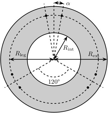
Figure 4: Schematic of the bottom plates with all the parameters
The goal is to choose \(\alpha\), \(\beta\), \(R_\text{leg, t}\) and \(R_\text{leg, b}\) in such a way that the configuration is cubic.
The configuration is cubic if: \[ \overrightarrow{a_i b_i} \cdot \overrightarrow{a_j b_j} = 0, \ \forall i, j = [1, \hdots, 6], i \ne j \]
Lets express \(a_i\), \(b_i\) and \(a_j\):
\begin{equation*} a_1 = \begin{bmatrix}R_{\text{leg,b}} \cos(120 - \alpha) \\ R_{\text{leg,b}} \cos(120 - \alpha) \\ 0\end{bmatrix} ; \quad a_2 = \begin{bmatrix}R_{\text{leg,b}} \cos(120 + \alpha) \\ R_{\text{leg,b}} \cos(120 + \alpha) \\ 0\end{bmatrix} ; \quad \end{equation*} \begin{equation*} b_1 = \begin{bmatrix}R_{\text{leg,t}} \cos(120 - \beta) \\ R_{\text{leg,t}} \cos(120 - \beta\\ H\end{bmatrix} ; \quad b_2 = \begin{bmatrix}R_{\text{leg,t}} \cos(120 + \beta) \\ R_{\text{leg,t}} \cos(120 + \beta\\ H\end{bmatrix} ; \quad \end{equation*}\[ \overrightarrow{a_1 b_1} = b_1 - a_1 = \begin{bmatrix}R_{\text{leg}} \cos(120 - \alpha) \\ R_{\text{leg}} \cos(120 - \alpha) \\ 0\end{bmatrix}\]
5.2 Second attempt
We start with the point of a cube in space:
\begin{align*} [0, 0, 0] ; \ [0, 0, 1]; \ ... \end{align*}We also want the cube to point upward: \[ [1, 1, 1] \Rightarrow [0, 0, 1] \]
Then we have the direction of all the vectors expressed in the frame of the hexapod.
points = [0, 0, 0; ...
          0, 0, 1; ...
          0, 1, 0; ...
          0, 1, 1; ...
          1, 0, 0; ...
          1, 0, 1; ...
          1, 1, 0; ...
          1, 1, 1];
figure;
plot3(points(:,1), points(:,2), points(:,3), 'ko')
sx = cross([1, 1, 1], [1 0 0]);
sx = sx/norm(sx);

sy = -cross(sx, [1, 1, 1]);
sy = sy/norm(sy);

sz = [1, 1, 1];
sz = sz/norm(sz);

R = [sx', sy', sz']';
cube = zeros(size(points));
for i = 1:size(points, 1)
  cube(i, :) = R * points(i, :)';
end
figure;
hold on;
plot3(points(:,1), points(:,2), points(:,3), 'ko');
plot3(cube(:,1), cube(:,2), cube(:,3), 'ro');
hold off;
Now we plot the legs of the hexapod.
leg_indices = [3, 4; ...
               2, 4; ...
               2, 6; ...
               5, 6; ...
               5, 7; ...
               3, 7]

figure;
hold on;
for i = 1:6
  plot3(cube(leg_indices(i, :),1), cube(leg_indices(i, :),2), cube(leg_indices(i, :),3), '-');
end
hold off;
Vectors are:
legs = zeros(6, 3);
legs_start = zeros(6, 3);

for i = 1:6
  legs(i, :) = cube(leg_indices(i, 2), :) - cube(leg_indices(i, 1), :);
  legs_start(i, :) = cube(leg_indices(i, 1), :)
end
We now have the orientation of each leg.
We here want to see if the position of the "slice" changes something.
Let's first estimate the maximum height of the Stewart platform.
Hmax = cube(4, 3) - cube(2, 3);
Let's then estimate the middle position of the platform
Hmid = cube(8, 3)/2;
5.3 Generate the Stewart platform for a Cubic configuration
First we defined the height of the Hexapod.
H = Hmax/2;
Zs = 1.2*cube(2, 3); % Height of the fixed platform
Ze = Zs + H; % Height of the mobile platform
We now determine the location of the joints on the fixed platform.
Aa = zeros(6, 3);
for i = 1:6
  t = (Zs-legs_start(i, 3))/(legs(i, 3));
  Aa(i, :) = legs_start(i, :) + t*legs(i, :);
end
And the location of the joints on the mobile platform
Ab = zeros(6, 3);
for i = 1:6
  t = (Ze-legs_start(i, 3))/(legs(i, 3));
  Ab(i, :) = legs_start(i, :) + t*legs(i, :);
end
And we plot the legs.
figure;
hold on;
for i = 1:6
  plot3([Ab(i, 1),Aa(i, 1)], [Ab(i, 2),Aa(i, 2)], [Ab(i, 3),Aa(i, 3)], 'k-');
end
hold off;
xlim([-1, 1]);
ylim([-1, 1]);
zlim([0, 2]);
Bibliography
- [geng94_six_degree_of_freed_activ] Geng & Haynes, Six Degree-Of-Freedom Active Vibration Control Using the Stewart Platforms, IEEE Transactions on Control Systems Technology, 2(1), 45-53 (1994). link. doi.
- [jafari03_orthog_gough_stewar_platf_microm] Jafari & McInroy, Orthogonal Gough-Stewart Platforms for Micromanipulation, IEEE Transactions on Robotics and Automation, 19(4), 595-603 (2003). link. doi.
- [preumont07_six_axis_singl_stage_activ] Preumont, Horodinca, Romanescu, de, Marneffe, Avraam, Deraemaeker, Bossens, & Abu Hanieh, A Six-Axis Single-Stage Active Vibration Isolator Based on Stewart Platform, Journal of Sound and Vibration, 300(3-5), 644-661 (2007). link. doi.