Stewart Platform - Definition of the Architecture
Table of Contents
- 1. Procedure
- 2. Matlab Code
- 3.
initializeFramesPositions: Initialize the positions of frames {A}, {B}, {F} and {M} - 4. Initialize the position of the Joints
- 5.
computeJointsPose: Compute the Pose of the Joints - 6.
initializeStrutDynamics: Add Stiffness and Damping properties of each strut - 7.
computeJacobian: Compute the Jacobian Matrix - 8. Initialize the Geometry of the Mechanical Elements
- 9.
initializeStewartPose: Determine the initial stroke in each leg to have the wanted pose - 10. Utility Functions
- 11. Other Elements
Stewart platforms are generated in multiple steps.
We define 4 important frames:
- \(\{F\}\): Frame fixed to the Fixed base and located at the center of its bottom surface. This is used to fix the Stewart platform to some support.
- \(\{M\}\): Frame fixed to the Moving platform and located at the center of its top surface. This is used to place things on top of the Stewart platform.
- \(\{A\}\): Frame fixed to the fixed base. It defined the center of rotation of the moving platform.
- \(\{B\}\): Frame fixed to the moving platform. The motion of the moving platforms and forces applied to it are defined with respect to this frame \(\{B\}\).
Then, we define the location of the spherical joints:
- \(\bm{a}_{i}\) are the position of the spherical joints fixed to the fixed base
- \(\bm{b}_{i}\) are the position of the spherical joints fixed to the moving platform
We define the rest position of the Stewart platform:
- For simplicity, we suppose that the fixed base and the moving platform are parallel and aligned with the vertical axis at their rest position.
- Thus, to define the rest position of the Stewart platform, we just have to defined its total height \(H\). \(H\) corresponds to the distance from the bottom of the fixed base to the top of the moving platform.
From \(\bm{a}_{i}\) and \(\bm{b}_{i}\), we can determine the length and orientation of each strut:
- \(l_{i}\) is the length of the strut
- \({}^{A}\hat{\bm{s}}_{i}\) is the unit vector align with the strut
The position of the Spherical joints can be computed using various methods:
- Cubic configuration
- Circular configuration
- Arbitrary position
- These methods should be easily scriptable and corresponds to specific functions that returns \({}^{F}\bm{a}_{i}\) and \({}^{M}\bm{b}_{i}\). The input of these functions are the parameters corresponding to the wanted geometry.
For Simscape, we need:
- The position and orientation of each spherical joint fixed to the fixed base: \({}^{F}\bm{a}_{i}\) and \({}^{F}\bm{R}_{a_{i}}\)
- The position and orientation of each spherical joint fixed to the moving platform: \({}^{M}\bm{b}_{i}\) and \({}^{M}\bm{R}_{b_{i}}\)
- The rest length of each strut: \(l_{i}\)
- The stiffness and damping of each actuator: \(k_{i}\) and \(c_{i}\)
- The position of the frame \(\{A\}\) with respect to the frame \(\{F\}\): \({}^{F}\bm{O}_{A}\)
- The position of the frame \(\{B\}\) with respect to the frame \(\{M\}\): \({}^{M}\bm{O}_{B}\)
1 Procedure
The procedure to define the Stewart platform is the following:
- Define the initial position of frames {A}, {B}, {F} and {M}.
We do that using the
initializeFramesPositionsfunction. We have to specify the total height of the Stewart platform \(H\) and the position \({}^{M}O_{B}\) of {B} with respect to {M}. - Compute the positions of joints \({}^{F}a_{i}\) and \({}^{M}b_{i}\).
We can do that using various methods depending on the wanted architecture:
generateCubicConfigurationpermits to generate a cubic configuration
- Compute the position and orientation of the joints with respect to the fixed base and the moving platform.
This is done with the
computeJointsPosefunction. - Define the dynamical properties of the Stewart platform. The output are the stiffness and damping of each strut \(k_{i}\) and \(c_{i}\). This can be done we simply choosing directly the stiffness and damping of each strut. The stiffness and damping of each actuator can also be determine from the wanted stiffness of the Stewart platform for instance.
- Define the mass and inertia of each element of the Stewart platform.
By following this procedure, we obtain a Matlab structure stewart that contains all the information for the Simscape model and for further analysis.
2 Matlab Code
2.1 Simscape Model
open('stewart_platform.slx')
2.2 Test the functions
stewart = initializeFramesPositions('H', 90e-3, 'MO_B', 45e-3);
% stewart = generateCubicConfiguration(stewart, 'Hc', 60e-3, 'FOc', 45e-3, 'FHa', 5e-3, 'MHb', 5e-3);
stewart = generateGeneralConfiguration(stewart);
stewart = computeJointsPose(stewart);
stewart = initializeStrutDynamics(stewart, 'Ki', 1e6*ones(6,1), 'Ci', 1e2*ones(6,1));
stewart = initializeCylindricalPlatforms(stewart);
stewart = initializeCylindricalStruts(stewart);
stewart = computeJacobian(stewart);
stewart = initializeStewartPose(stewart, 'AP', [0;0;0.01], 'ARB', eye(3));

[Li, dLi] = inverseKinematics(stewart, 'AP', [0;0;0.00001], 'ARB', eye(3));
[P, R] = forwardKinematicsApprox(stewart, 'dL', dLi);
3 initializeFramesPositions: Initialize the positions of frames {A}, {B}, {F} and {M}
This Matlab function is accessible here.
3.1 Function description
function [stewart] = initializeFramesPositions(args)
% initializeFramesPositions - Initialize the positions of frames {A}, {B}, {F} and {M}
%
% Syntax: [stewart] = initializeFramesPositions(args)
%
% Inputs:
%    - args - Can have the following fields:
%        - H    [1x1] - Total Height of the Stewart Platform (height from {F} to {M}) [m]
%        - MO_B [1x1] - Height of the frame {B} with respect to {M} [m]
%
% Outputs:
%    - stewart - A structure with the following fields:
%        - H    [1x1] - Total Height of the Stewart Platform [m]
%        - FO_M [3x1] - Position of {M} with respect to {F} [m]
%        - MO_B [3x1] - Position of {B} with respect to {M} [m]
%        - FO_A [3x1] - Position of {A} with respect to {F} [m]
3.2 Documentation
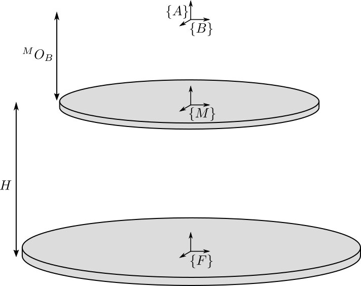
Figure 1: Definition of the position of the frames
3.3 Optional Parameters
arguments
    args.H    (1,1) double {mustBeNumeric, mustBePositive} = 90e-3
    args.MO_B (1,1) double {mustBeNumeric} = 50e-3
end
3.4 Initialize the Stewart structure
stewart = struct();
3.5 Compute the position of each frame
stewart.H = args.H; % Total Height of the Stewart Platform [m]

stewart.FO_M = [0; 0; stewart.H]; % Position of {M} with respect to {F} [m]

stewart.MO_B = [0; 0; args.MO_B]; % Position of {B} with respect to {M} [m]

stewart.FO_A = stewart.MO_B + stewart.FO_M; % Position of {A} with respect to {F} [m]
4 Initialize the position of the Joints
4.1 generateCubicConfiguration: Generate a Cubic Configuration
This Matlab function is accessible here.
4.1.1 Function description
function [stewart] = generateCubicConfiguration(stewart, args)
% generateCubicConfiguration - Generate a Cubic Configuration
%
% Syntax: [stewart] = generateCubicConfiguration(stewart, args)
%
% Inputs:
%    - stewart - A structure with the following fields
%        - H   [1x1] - Total height of the platform [m]
%    - args - Can have the following fields:
%        - Hc  [1x1] - Height of the "useful" part of the cube [m]
%        - FOc [1x1] - Height of the center of the cube with respect to {F} [m]
%        - FHa [1x1] - Height of the plane joining the points ai with respect to the frame {F} [m]
%        - MHb [1x1] - Height of the plane joining the points bi with respect to the frame {M} [m]
%
% Outputs:
%    - stewart - updated Stewart structure with the added fields:
%        - Fa  [3x6] - Its i'th column is the position vector of joint ai with respect to {F}
%        - Mb  [3x6] - Its i'th column is the position vector of joint bi with respect to {M}
4.1.2 Documentation
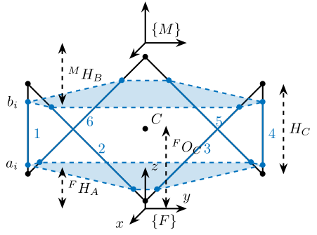
Figure 2: Cubic Configuration
4.1.3 Optional Parameters
arguments
    stewart
    args.Hc  (1,1) double {mustBeNumeric, mustBePositive} = 60e-3
    args.FOc (1,1) double {mustBeNumeric} = 50e-3
    args.FHa (1,1) double {mustBeNumeric, mustBePositive} = 15e-3
    args.MHb (1,1) double {mustBeNumeric, mustBePositive} = 15e-3
end
4.1.4 Position of the Cube
We define the useful points of the cube with respect to the Cube’s center. \({}^{C}C\) are the 6 vertices of the cubes expressed in a frame {C} which is located at the center of the cube and aligned with {F} and {M}.
sx = [ 2; -1; -1];
sy = [ 0;  1; -1];
sz = [ 1;  1;  1];

R = [sx, sy, sz]./vecnorm([sx, sy, sz]);

L = args.Hc*sqrt(3);

Cc = R'*[[0;0;L],[L;0;L],[L;0;0],[L;L;0],[0;L;0],[0;L;L]] - [0;0;1.5*args.Hc];

CCf = [Cc(:,1), Cc(:,3), Cc(:,3), Cc(:,5), Cc(:,5), Cc(:,1)]; % CCf(:,i) corresponds to the bottom cube's vertice corresponding to the i'th leg
CCm = [Cc(:,2), Cc(:,2), Cc(:,4), Cc(:,4), Cc(:,6), Cc(:,6)]; % CCm(:,i) corresponds to the top cube's vertice corresponding to the i'th leg
4.1.5 Compute the pose
We can compute the vector of each leg \({}^{C}\hat{\bm{s}}_{i}\) (unit vector from \({}^{C}C_{f}\) to \({}^{C}C_{m}\)).
CSi = (CCm - CCf)./vecnorm(CCm - CCf);
We now which to compute the position of the joints \(a_{i}\) and \(b_{i}\).
stewart.Fa = CCf + [0; 0; args.FOc] + ((args.FHa-(args.FOc-args.Hc/2))./CSi(3,:)).*CSi;
stewart.Mb = CCf + [0; 0; args.FOc-stewart.H] + ((stewart.H-args.MHb-(args.FOc-args.Hc/2))./CSi(3,:)).*CSi;
4.2 generateGeneralConfiguration: Generate a Very General Configuration
This Matlab function is accessible here.
4.2.1 Function description
function [stewart] = generateGeneralConfiguration(stewart, args)
% generateGeneralConfiguration - Generate a Very General Configuration
%
% Syntax: [stewart] = generateGeneralConfiguration(stewart, args)
%
% Inputs:
%    - args - Can have the following fields:
%        - FH  [1x1] - Height of the position of the fixed joints with respect to the frame {F} [m]
%        - FR  [1x1] - Radius of the position of the fixed joints in the X-Y [m]
%        - FTh [6x1] - Angles of the fixed joints in the X-Y plane with respect to the X axis [rad]
%        - MH  [1x1] - Height of the position of the mobile joints with respect to the frame {M} [m]
%        - FR  [1x1] - Radius of the position of the mobile joints in the X-Y [m]
%        - MTh [6x1] - Angles of the mobile joints in the X-Y plane with respect to the X axis [rad]
%
% Outputs:
%    - stewart - updated Stewart structure with the added fields:
%        - Fa  [3x6] - Its i'th column is the position vector of joint ai with respect to {F}
%        - Mb  [3x6] - Its i'th column is the position vector of joint bi with respect to {M}
4.2.2 Documentation
Joints are positions on a circle centered with the Z axis of {F} and {M} and at a chosen distance from {F} and {M}. The radius of the circles can be chosen as well as the angles where the joints are located.
4.2.3 Optional Parameters
arguments
    stewart
    args.FH  (1,1) double {mustBeNumeric, mustBePositive} = 15e-3
    args.FR  (1,1) double {mustBeNumeric, mustBePositive} = 115e-3;
    args.FTh (6,1) double {mustBeNumeric} = [-10, 10, 120-10, 120+10, 240-10, 240+10]*(pi/180);
    args.MH  (1,1) double {mustBeNumeric, mustBePositive} = 15e-3
    args.MR  (1,1) double {mustBeNumeric, mustBePositive} = 90e-3;
    args.MTh (6,1) double {mustBeNumeric} = [-60+10, 60-10, 60+10, 180-10, 180+10, -60-10]*(pi/180);
end
4.2.4 Compute the pose
stewart.Fa = zeros(3,6);
stewart.Mb = zeros(3,6);
for i = 1:6
  stewart.Fa(:,i) = [args.FR*cos(args.FTh(i)); args.FR*sin(args.FTh(i)); args.FH];
  stewart.Mb(:,i) = [args.MR*cos(args.MTh(i)); args.MR*sin(args.MTh(i)); -args.MH];
end
5 computeJointsPose: Compute the Pose of the Joints
This Matlab function is accessible here.
5.1 Function description
function [stewart] = computeJointsPose(stewart)
% computeJointsPose -
%
% Syntax: [stewart] = computeJointsPose(stewart)
%
% Inputs:
%    - stewart - A structure with the following fields
%        - Fa   [3x6] - Its i'th column is the position vector of joint ai with respect to {F}
%        - Mb   [3x6] - Its i'th column is the position vector of joint bi with respect to {M}
%        - FO_A [3x1] - Position of {A} with respect to {F}
%        - MO_B [3x1] - Position of {B} with respect to {M}
%        - FO_M [3x1] - Position of {M} with respect to {F}
%
% Outputs:
%    - stewart - A structure with the following added fields
%        - Aa  [3x6]   - The i'th column is the position of ai with respect to {A}
%        - Ab  [3x6]   - The i'th column is the position of bi with respect to {A}
%        - Ba  [3x6]   - The i'th column is the position of ai with respect to {B}
%        - Bb  [3x6]   - The i'th column is the position of bi with respect to {B}
%        - l   [6x1]   - The i'th element is the initial length of strut i
%        - As  [3x6]   - The i'th column is the unit vector of strut i expressed in {A}
%        - Bs  [3x6]   - The i'th column is the unit vector of strut i expressed in {B}
%        - FRa [3x3x6] - The i'th 3x3 array is the rotation matrix to orientate the bottom of the i'th strut from {F}
%        - MRb [3x3x6] - The i'th 3x3 array is the rotation matrix to orientate the top of the i'th strut from {M}
5.2 Documentation
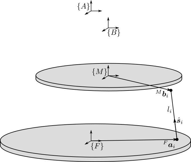
Figure 3: Position and orientation of the struts
5.3 Compute the position of the Joints
stewart.Aa = stewart.Fa - repmat(stewart.FO_A, [1, 6]);
stewart.Bb = stewart.Mb - repmat(stewart.MO_B, [1, 6]);

stewart.Ab = stewart.Bb - repmat(-stewart.MO_B-stewart.FO_M+stewart.FO_A, [1, 6]);
stewart.Ba = stewart.Aa - repmat( stewart.MO_B+stewart.FO_M-stewart.FO_A, [1, 6]);
5.4 Compute the strut length and orientation
stewart.As = (stewart.Ab - stewart.Aa)./vecnorm(stewart.Ab - stewart.Aa); % As_i is the i'th vector of As

stewart.l = vecnorm(stewart.Ab - stewart.Aa)';
stewart.Bs = (stewart.Bb - stewart.Ba)./vecnorm(stewart.Bb - stewart.Ba);
5.5 Compute the orientation of the Joints
stewart.FRa = zeros(3,3,6);
stewart.MRb = zeros(3,3,6);

for i = 1:6
  stewart.FRa(:,:,i) = [cross([0;1;0], stewart.As(:,i)) , cross(stewart.As(:,i), cross([0;1;0], stewart.As(:,i))) , stewart.As(:,i)];
  stewart.FRa(:,:,i) = stewart.FRa(:,:,i)./vecnorm(stewart.FRa(:,:,i));

  stewart.MRb(:,:,i) = [cross([0;1;0], stewart.Bs(:,i)) , cross(stewart.Bs(:,i), cross([0;1;0], stewart.Bs(:,i))) , stewart.Bs(:,i)];
  stewart.MRb(:,:,i) = stewart.MRb(:,:,i)./vecnorm(stewart.MRb(:,:,i));
end
6 initializeStrutDynamics: Add Stiffness and Damping properties of each strut
This Matlab function is accessible here.
6.1 Function description
function [stewart] = initializeStrutDynamics(stewart, args)
% initializeStrutDynamics - Add Stiffness and Damping properties of each strut
%
% Syntax: [stewart] = initializeStrutDynamics(args)
%
% Inputs:
%    - args - Structure with the following fields:
%        - Ki [6x1] - Stiffness of each strut [N/m]
%        - Ci [6x1] - Damping of each strut [N/(m/s)]
%
% Outputs:
%    - stewart - updated Stewart structure with the added fields:
%        - Ki [6x1] - Stiffness of each strut [N/m]
%        - Ci [6x1] - Damping of each strut [N/(m/s)]
6.2 Optional Parameters
arguments
    stewart
    args.Ki (6,1) double {mustBeNumeric, mustBePositive} = 1e6*ones(6,1)
    args.Ci (6,1) double {mustBeNumeric, mustBePositive} = 1e1*ones(6,1)
end
6.3 Add Stiffness and Damping properties of each strut
stewart.Ki = args.Ki;
stewart.Ci = args.Ci;
7 computeJacobian: Compute the Jacobian Matrix
This Matlab function is accessible here.
7.1 Function description
function [stewart] = computeJacobian(stewart)
% computeJacobian -
%
% Syntax: [stewart] = computeJacobian(stewart)
%
% Inputs:
%    - stewart - With at least the following fields:
%        - As [3x6] - The 6 unit vectors for each strut expressed in {A}
%        - Ab [3x6] - The 6 position of the joints bi expressed in {A}
%
% Outputs:
%    - stewart - With the 3 added field:
%        - J [6x6] - The Jacobian Matrix
%        - K [6x6] - The Stiffness Matrix
%        - C [6x6] - The Compliance Matrix
7.2 Compute Jacobian Matrix
stewart.J = [stewart.As' , cross(stewart.Ab, stewart.As)'];
7.3 Compute Stiffness Matrix
stewart.K = stewart.J'*diag(stewart.Ki)*stewart.J;
7.4 Compute Compliance Matrix
stewart.C = inv(stewart.K);
8 Initialize the Geometry of the Mechanical Elements
8.1 initializeCylindricalPlatforms: Initialize the geometry of the Fixed and Mobile Platforms
This Matlab function is accessible here.
8.1.1 Function description
function [stewart] = initializeCylindricalPlatforms(stewart, args)
% initializeCylindricalPlatforms - Initialize the geometry of the Fixed and Mobile Platforms
%
% Syntax: [stewart] = initializeCylindricalPlatforms(args)
%
% Inputs:
%    - args - Structure with the following fields:
%        - Fpm [1x1] - Fixed Platform Mass [kg]
%        - Fph [1x1] - Fixed Platform Height [m]
%        - Fpr [1x1] - Fixed Platform Radius [m]
%        - Mpm [1x1] - Mobile Platform Mass [kg]
%        - Mph [1x1] - Mobile Platform Height [m]
%        - Mpr [1x1] - Mobile Platform Radius [m]
%
% Outputs:
%    - stewart - updated Stewart structure with the added fields:
%      - platforms [struct] - structure with the following fields:
%        - Fpm [1x1] - Fixed Platform Mass [kg]
%        - Msi [3x3] - Mobile Platform Inertia matrix [kg*m^2]
%        - Fph [1x1] - Fixed Platform Height [m]
%        - Fpr [1x1] - Fixed Platform Radius [m]
%        - Mpm [1x1] - Mobile Platform Mass [kg]
%        - Fsi [3x3] - Fixed Platform Inertia matrix [kg*m^2]
%        - Mph [1x1] - Mobile Platform Height [m]
%        - Mpr [1x1] - Mobile Platform Radius [m]
8.1.2 Optional Parameters
arguments
    stewart
    args.Fpm (1,1) double {mustBeNumeric, mustBePositive} = 1
    args.Fph (1,1) double {mustBeNumeric, mustBePositive} = 10e-3
    args.Fpr (1,1) double {mustBeNumeric, mustBePositive} = 125e-3
    args.Mpm (1,1) double {mustBeNumeric, mustBePositive} = 1
    args.Mph (1,1) double {mustBeNumeric, mustBePositive} = 10e-3
    args.Mpr (1,1) double {mustBeNumeric, mustBePositive} = 100e-3
end
8.1.3 Create the platforms struct
platforms = struct();

platforms.Fpm = args.Fpm;
platforms.Fph = args.Fph;
platforms.Fpr = args.Fpr;
platforms.Fpi = diag([1/12 * platforms.Fpm * (3*platforms.Fpr^2 + platforms.Fph^2), ...
                      1/12 * platforms.Fpm * (3*platforms.Fpr^2 + platforms.Fph^2), ...
                      1/2  * platforms.Fpm * platforms.Fpr^2]);

platforms.Mpm = args.Mpm;
platforms.Mph = args.Mph;
platforms.Mpr = args.Mpr;
platforms.Mpi = diag([1/12 * platforms.Mpm * (3*platforms.Mpr^2 + platforms.Mph^2), ...
                      1/12 * platforms.Mpm * (3*platforms.Mpr^2 + platforms.Mph^2), ...
                      1/2  * platforms.Mpm * platforms.Mpr^2]);
8.1.4 Save the platforms struct
stewart.platforms = platforms;
8.2 initializeCylindricalStruts: Define the mass and moment of inertia of cylindrical struts
This Matlab function is accessible here.
8.2.1 Function description
function [stewart] = initializeCylindricalStruts(stewart, args)
% initializeCylindricalStruts - Define the mass and moment of inertia of cylindrical struts
%
% Syntax: [stewart] = initializeCylindricalStruts(args)
%
% Inputs:
%    - args - Structure with the following fields:
%        - Fsm [1x1] - Mass of the Fixed part of the struts [kg]
%        - Fsh [1x1] - Height of cylinder for the Fixed part of the struts [m]
%        - Fsr [1x1] - Radius of cylinder for the Fixed part of the struts [m]
%        - Msm [1x1] - Mass of the Mobile part of the struts [kg]
%        - Msh [1x1] - Height of cylinder for the Mobile part of the struts [m]
%        - Msr [1x1] - Radius of cylinder for the Mobile part of the struts [m]
%
% Outputs:
%    - stewart - updated Stewart structure with the added fields:
%      - struts [struct] - structure with the following fields:
%        - Fsm [6x1]   - Mass of the Fixed part of the struts [kg]
%        - Fsi [3x3x6] - Moment of Inertia for the Fixed part of the struts [kg*m^2]
%        - Msm [6x1]   - Mass of the Mobile part of the struts [kg]
%        - Msi [3x3x6] - Moment of Inertia for the Mobile part of the struts [kg*m^2]
%        - Fsh [6x1]   - Height of cylinder for the Fixed part of the struts [m]
%        - Fsr [6x1]   - Radius of cylinder for the Fixed part of the struts [m]
%        - Msh [6x1]   - Height of cylinder for the Mobile part of the struts [m]
%        - Msr [6x1]   - Radius of cylinder for the Mobile part of the struts [m]
8.2.2 Optional Parameters
arguments
    stewart
    args.Fsm (1,1) double {mustBeNumeric, mustBePositive} = 0.1
    args.Fsh (1,1) double {mustBeNumeric, mustBePositive} = 50e-3
    args.Fsr (1,1) double {mustBeNumeric, mustBePositive} = 5e-3
    args.Msm (1,1) double {mustBeNumeric, mustBePositive} = 0.1
    args.Msh (1,1) double {mustBeNumeric, mustBePositive} = 50e-3
    args.Msr (1,1) double {mustBeNumeric, mustBePositive} = 5e-3
end
8.2.3 Create the struts structure
struts = struct();

struts.Fsm = ones(6,1).*args.Fsm;
struts.Msm = ones(6,1).*args.Msm;

struts.Fsh = ones(6,1).*args.Fsh;
struts.Fsr = ones(6,1).*args.Fsr;
struts.Msh = ones(6,1).*args.Msh;
struts.Msr = ones(6,1).*args.Msr;

struts.Fsi = zeros(3, 3, 6);
struts.Msi = zeros(3, 3, 6);
for i = 1:6
  struts.Fsi(:,:,i) = diag([1/12 * struts.Fsm(i) * (3*struts.Fsr(i)^2 + struts.Fsh(i)^2), ...
                            1/12 * struts.Fsm(i) * (3*struts.Fsr(i)^2 + struts.Fsh(i)^2), ...
                            1/2  * struts.Fsm(i) * struts.Fsr(i)^2]);
  struts.Msi(:,:,i) = diag([1/12 * struts.Msm(i) * (3*struts.Msr(i)^2 + struts.Msh(i)^2), ...
                            1/12 * struts.Msm(i) * (3*struts.Msr(i)^2 + struts.Msh(i)^2), ...
                            1/2  * struts.Msm(i) * struts.Msr(i)^2]);
end
stewart.struts = struts;
9 initializeStewartPose: Determine the initial stroke in each leg to have the wanted pose
This Matlab function is accessible here.
9.1 Function description
function [stewart] = initializeStewartPose(stewart, args)
% initializeStewartPose - Determine the initial stroke in each leg to have the wanted pose
%                         It uses the inverse kinematic
%
% Syntax: [stewart] = initializeStewartPose(stewart, args)
%
% Inputs:
%    - stewart - A structure with the following fields
%        - Aa   [3x6] - The positions ai expressed in {A}
%        - Bb   [3x6] - The positions bi expressed in {B}
%    - args - Can have the following fields:
%        - AP   [3x1] - The wanted position of {B} with respect to {A}
%        - ARB  [3x3] - The rotation matrix that gives the wanted orientation of {B} with respect to {A}
%
% Outputs:
%    - stewart - updated Stewart structure with the added fields:
%      - dLi[6x1] - The 6 needed displacement of the struts from the initial position in [m] to have the wanted pose of {B} w.r.t. {A}
9.2 Optional Parameters
arguments
    stewart
    args.AP  (3,1) double {mustBeNumeric} = zeros(3,1)
    args.ARB (3,3) double {mustBeNumeric} = eye(3)
end
9.3 Use the Inverse Kinematic function
[Li, dLi] = inverseKinematics(stewart, 'AP', args.AP, 'ARB', args.ARB);

stewart.dLi = dLi;
10 Utility Functions
10.1 inverseKinematics: Compute Inverse Kinematics
This Matlab function is accessible here.
10.1.1 Function description
function [Li, dLi] = inverseKinematics(stewart, args)
% inverseKinematics - Compute the needed length of each strut to have the wanted position and orientation of {B} with respect to {A}
%
% Syntax: [stewart] = inverseKinematics(stewart)
%
% Inputs:
%    - stewart - A structure with the following fields
%        - Aa   [3x6] - The positions ai expressed in {A}
%        - Bb   [3x6] - The positions bi expressed in {B}
%    - args - Can have the following fields:
%        - AP   [3x1] - The wanted position of {B} with respect to {A}
%        - ARB  [3x3] - The rotation matrix that gives the wanted orientation of {B} with respect to {A}
%
% Outputs:
%    - Li   [6x1] - The 6 needed length of the struts in [m] to have the wanted pose of {B} w.r.t. {A}
%    - dLi  [6x1] - The 6 needed displacement of the struts from the initial position in [m] to have the wanted pose of {B} w.r.t. {A}
10.1.2 Optional Parameters
arguments
    stewart
    args.AP  (3,1) double {mustBeNumeric} = zeros(3,1)
    args.ARB (3,3) double {mustBeNumeric} = eye(3)
end
10.1.3 Theory
For inverse kinematic analysis, it is assumed that the position \({}^A\bm{P}\) and orientation of the moving platform \({}^A\bm{R}_B\) are given and the problem is to obtain the joint variables, namely, \(\bm{L} = [l_1, l_2, \dots, l_6]^T\).
From the geometry of the manipulator, the loop closure for each limb, \(i = 1, 2, \dots, 6\) can be written as
\begin{align*} l_i {}^A\hat{\bm{s}}_i &= {}^A\bm{A} + {}^A\bm{b}_i - {}^A\bm{a}_i \\ &= {}^A\bm{A} + {}^A\bm{R}_b {}^B\bm{b}_i - {}^A\bm{a}_i \end{align*}To obtain the length of each actuator and eliminate \(\hat{\bm{s}}_i\), it is sufficient to dot multiply each side by itself:
\begin{equation} l_i^2 \left[ {}^A\hat{\bm{s}}_i^T {}^A\hat{\bm{s}}_i \right] = \left[ {}^A\bm{P} + {}^A\bm{R}_B {}^B\bm{b}_i - {}^A\bm{a}_i \right]^T \left[ {}^A\bm{P} + {}^A\bm{R}_B {}^B\bm{b}_i - {}^A\bm{a}_i \right] \end{equation}Hence, for \(i = 1, 2, \dots, 6\), each limb length can be uniquely determined by:
\begin{equation} l_i = \sqrt{{}^A\bm{P}^T {}^A\bm{P} + {}^B\bm{b}_i^T {}^B\bm{b}_i + {}^A\bm{a}_i^T {}^A\bm{a}_i - 2 {}^A\bm{P}^T {}^A\bm{a}_i + 2 {}^A\bm{P}^T \left[{}^A\bm{R}_B {}^B\bm{b}_i\right] - 2 \left[{}^A\bm{R}_B {}^B\bm{b}_i\right]^T {}^A\bm{a}_i} \end{equation}If the position and orientation of the moving platform lie in the feasible workspace of the manipulator, one unique solution to the limb length is determined by the above equation. Otherwise, when the limbs’ lengths derived yield complex numbers, then the position or orientation of the moving platform is not reachable.
10.1.4 Compute
Li = sqrt(args.AP'*args.AP + diag(stewart.Bb'*stewart.Bb) + diag(stewart.Aa'*stewart.Aa) - (2*args.AP'*stewart.Aa)' + (2*args.AP'*(args.ARB*stewart.Bb))' - diag(2*(args.ARB*stewart.Bb)'*stewart.Aa));
dLi = Li-stewart.l;
10.2 forwardKinematicsApprox: Compute the Forward Kinematics
This Matlab function is accessible here.
10.2.1 Function description
function [P, R] = forwardKinematicsApprox(stewart, args)
% forwardKinematicsApprox - Computed the approximate pose of {B} with respect to {A} from the length of each strut and using
%                           the Jacobian Matrix
%
% Syntax: [P, R] = forwardKinematicsApprox(stewart, args)
%
% Inputs:
%    - stewart - A structure with the following fields
%        - J  [6x6] - The Jacobian Matrix
%    - args - Can have the following fields:
%        - dL [6x1] - Displacement of each strut [m]
%
% Outputs:
%    - P  [3x1] - The estimated position of {B} with respect to {A}
%    - R  [3x3] - The estimated rotation matrix that gives the orientation of {B} with respect to {A}
10.2.2 Optional Parameters
arguments
    stewart
    args.dL (6,1) double {mustBeNumeric} = zeros(6,1)
end
10.2.3 Computation
From a small displacement of each strut \(d\bm{\mathcal{L}}\), we can compute the position and orientation of {B} with respect to {A} using the following formula: \[ d \bm{\mathcal{X}} = \bm{J}^{-1} d\bm{\mathcal{L}} \]
X = stewart.J\args.dL;
The position vector corresponds to the first 3 elements.
P = X(1:3);
The next 3 elements are the orientation of {B} with respect to {A} expressed using the screw axis.
theta = norm(X(4:6));
s = X(4:6)/theta;
We then compute the corresponding rotation matrix.
R = [s(1)^2*(1-cos(theta)) + cos(theta) ,        s(1)*s(2)*(1-cos(theta)) - s(3)*sin(theta), s(1)*s(3)*(1-cos(theta)) + s(2)*sin(theta);
     s(2)*s(1)*(1-cos(theta)) + s(3)*sin(theta), s(2)^2*(1-cos(theta)) + cos(theta),         s(2)*s(3)*(1-cos(theta)) - s(1)*sin(theta);
     s(3)*s(1)*(1-cos(theta)) - s(2)*sin(theta), s(3)*s(2)*(1-cos(theta)) + s(1)*sin(theta), s(3)^2*(1-cos(theta)) + cos(theta)];
11 Other Elements
11.1 Z-Axis Geophone
This Matlab function is accessible here.
function [geophone] = initializeZAxisGeophone(args)
    arguments
        args.mass (1,1) double {mustBeNumeric, mustBePositive} = 1e-3 % [kg]
        args.freq (1,1) double {mustBeNumeric, mustBePositive} = 1    % [Hz]
    end

    %%
    geophone.m = args.mass;

    %% The Stiffness is set to have the damping resonance frequency
    geophone.k = geophone.m * (2*pi*args.freq)^2;

    %% We set the damping value to have critical damping
    geophone.c = 2*sqrt(geophone.m * geophone.k);

    %% Save
    save('./mat/geophone_z_axis.mat', 'geophone');
end
11.2 Z-Axis Accelerometer
This Matlab function is accessible here.
function [accelerometer] = initializeZAxisAccelerometer(args)
    arguments
        args.mass (1,1) double {mustBeNumeric, mustBePositive} = 1e-3 % [kg]
        args.freq (1,1) double {mustBeNumeric, mustBePositive} = 5e3  % [Hz]
    end

    %%
    accelerometer.m = args.mass;

    %% The Stiffness is set to have the damping resonance frequency
    accelerometer.k = accelerometer.m * (2*pi*args.freq)^2;

    %% We set the damping value to have critical damping
    accelerometer.c = 2*sqrt(accelerometer.m * accelerometer.k);

    %% Gain correction of the accelerometer to have a unity gain until the resonance
    accelerometer.gain = -accelerometer.k/accelerometer.m;

    %% Save
    save('./mat/accelerometer_z_axis.mat', 'accelerometer');
end