Stewart Platform - Simscape Model
Table of Contents
1 Function description and arguments
The initializeHexapod function takes one structure that contains configurations for the hexapod and returns one structure representing the hexapod.
function [stewart] = initializeHexapod(opts_param)
Default values for opts.
opts = struct(...
    'height',  90,    ... % Height of the platform [mm]
    'density', 8000,  ... % Density of the material used for the hexapod [kg/m3]
    'k_ax',    1e8,   ... % Stiffness of each actuator [N/m]
    'c_ax',    1000,   ... % Damping of each actuator [N/(m/s)]
    'stroke',  50e-6, ... % Maximum stroke of each actuator [m]
    'name',    'stewart' ... % Name of the file
    );
Populate opts with input parameters
if exist('opts_param','var')
    for opt = fieldnames(opts_param)'
        opts.(opt{1}) = opts_param.(opt{1});
    end
end
2 Initialization of the stewart structure
We initialize the Stewart structure
stewart = struct();
And we defined its total height.
stewart.H = opts.height; % [mm]
3 Bottom Plate

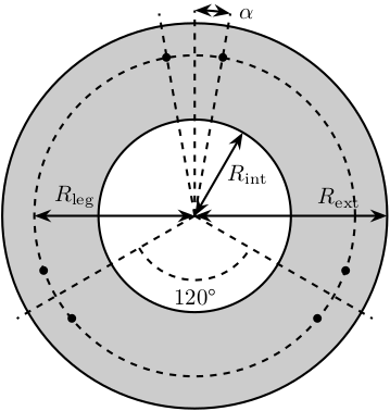
Figure 1: Schematic of the bottom plates with all the parameters
The bottom plate structure is initialized.
BP = struct();
We defined its internal radius (if there is a hole in the bottom plate) and its outer radius.
BP.Rint = 0;   % Internal Radius [mm]
BP.Rext = 150; % External Radius [mm]
We define its thickness.
BP.H = 10; % Thickness of the Bottom Plate [mm]
At which radius legs will be fixed and with that angle offset.
BP.Rleg  = 100; % Radius where the legs articulations are positionned [mm]
BP.alpha = 10;  % Angle Offset [deg]
We defined the density of the material of the bottom plate.
BP.density = opts.density; % Density of the material [kg/m3]
And its color.
BP.color = [0.7 0.7 0.7]; % Color [RGB]
Then the profile of the bottom plate is computed and will be used by Simscape
BP.shape = [BP.Rint BP.H; BP.Rint 0; BP.Rext 0; BP.Rext BP.H]; % [mm]
The structure is added to the stewart structure
stewart.BP = BP;
4 Top Plate
The top plate structure is initialized.
TP = struct();
We defined the internal and external radius of the top plate.
TP.Rint = 0;   % [mm]
TP.Rext = 100; % [mm]
The thickness of the top plate.
TP.H = 10; % [mm]
At which radius and angle are fixed the legs.
TP.Rleg   = 100; % Radius where the legs articulations are positionned [mm]
TP.alpha  = 20; % Angle [deg]
TP.dalpha = 0; % Angle Offset from 0 position [deg]
The density of its material.
TP.density = opts.density; % Density of the material [kg/m3]
Its color.
TP.color = [0.7 0.7 0.7]; % Color [RGB]
Then the shape of the top plate is computed
TP.shape = [TP.Rint TP.H; TP.Rint 0; TP.Rext 0; TP.Rext TP.H];
The structure is added to the stewart structure
stewart.TP = TP;
5 Legs

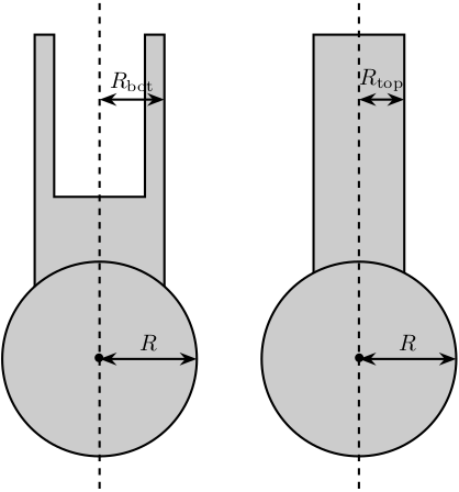
Figure 2: Schematic for the legs of the Stewart platform
The leg structure is initialized.
Leg = struct();
The maximum Stroke of each leg is defined.
Leg.stroke = opts.stroke; % [m]
The stiffness and damping of each leg are defined
Leg.k_ax = opts.k_ax; % Stiffness of each leg [N/m]
Leg.c_ax = opts.c_ax; % Damping of each leg [N/(m/s)]
The radius of the legs are defined
Leg.Rtop = 10; % Radius of the cylinder of the top part of the leg[mm]
Leg.Rbot = 12; % Radius of the cylinder of the bottom part of the leg [mm]
The density of its material.
Leg.density = opts.density; % Density of the material used for the legs [kg/m3]
Its color.
Leg.color = [0.5 0.5 0.5]; % Color of the top part of the leg [RGB]
The radius of spheres representing the ball joints are defined.
Leg.R = 1.3*Leg.Rbot; % Size of the sphere at the extremity of the leg [mm]
The structure is added to the stewart structure
stewart.Leg = Leg;
6 Ball Joints

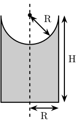
Figure 3: Schematic of the support for the ball joints
SP is the structure representing the support for the ball joints at the extremity of each leg.
The SP structure is initialized.
SP = struct();
We can define its rotational stiffness and damping. For now, we use perfect joints.
SP.k = 0; % [N*m/deg]
SP.c = 0; % [N*m/deg]
Its height is defined
SP.H = 15; % [mm]
Its radius is based on the radius on the sphere at the end of the legs.
SP.R = Leg.R; % [mm]
SP.section = [0    SP.H-SP.R;
              0    0;
              SP.R 0;
              SP.R SP.H];
The density of its material is defined.
SP.density = opts.density; % [kg/m^3]
Its color is defined.
SP.color = [0.7 0.7 0.7]; % [RGB]
The structure is added to the Hexapod structure
stewart.SP = SP;
7 More parameters are initialized
stewart = initializeParameters(stewart);
8 Save the Stewart Structure
save('./mat/stewart.mat', 'stewart')
9 initializeParameters Function
function [stewart] = initializeParameters(stewart)
We first compute \([a_1, a_2, a_3, a_4, a_5, a_6]^T\) and \([b_1, b_2, b_3, b_4, b_5, b_6]^T\).
stewart.Aa = zeros(6, 3); % [mm]
stewart.Ab = zeros(6, 3); % [mm]
stewart.Bb = zeros(6, 3); % [mm]
for i = 1:3
    stewart.Aa(2*i-1,:) = [stewart.BP.Rleg*cos( pi/180*(120*(i-1) - stewart.BP.alpha) ), ...
                           stewart.BP.Rleg*sin( pi/180*(120*(i-1) - stewart.BP.alpha) ), ...
                           stewart.BP.H+stewart.SP.H];
    stewart.Aa(2*i,:)   = [stewart.BP.Rleg*cos( pi/180*(120*(i-1) + stewart.BP.alpha) ), ...
                           stewart.BP.Rleg*sin( pi/180*(120*(i-1) + stewart.BP.alpha) ), ...
                           stewart.BP.H+stewart.SP.H];

    stewart.Ab(2*i-1,:) = [stewart.TP.Rleg*cos( pi/180*(120*(i-1) + stewart.TP.dalpha - stewart.TP.alpha) ), ...
                           stewart.TP.Rleg*sin( pi/180*(120*(i-1) + stewart.TP.dalpha - stewart.TP.alpha) ), ...
                           stewart.H - stewart.TP.H - stewart.SP.H];
    stewart.Ab(2*i,:)   = [stewart.TP.Rleg*cos( pi/180*(120*(i-1) + stewart.TP.dalpha + stewart.TP.alpha) ), ...
                           stewart.TP.Rleg*sin( pi/180*(120*(i-1) + stewart.TP.dalpha + stewart.TP.alpha) ), ...
                           stewart.H - stewart.TP.H - stewart.SP.H];
end
stewart.Bb = stewart.Ab - stewart.H*[0,0,1];
Now, we compute the leg vectors \(\hat{s}_i\) and leg position \(l_i\): \[ b_i - a_i = l_i \hat{s}_i \]
We initialize \(l_i\) and \(\hat{s}_i\)
leg_length = zeros(6, 1); % [mm]
leg_vectors = zeros(6, 3);
We compute \(b_i - a_i\), and then:
\begin{align*} l_i &= \left|b_i - a_i\right| \\ \hat{s}_i &= \frac{b_i - a_i}{l_i} \end{align*}legs = stewart.Ab - stewart.Aa; for i = 1:6 leg_length(i) = norm(legs(i,:)); leg_vectors(i,:) = legs(i,:) / leg_length(i); end
Then the shape of the bottom leg is estimated
stewart.Leg.lenght = leg_length(1)/1.5;
stewart.Leg.shape.bot = ...
    [0                0; ...
     stewart.Leg.Rbot 0; ...
     stewart.Leg.Rbot stewart.Leg.lenght; ...
     stewart.Leg.Rtop stewart.Leg.lenght; ...
     stewart.Leg.Rtop 0.2*stewart.Leg.lenght; ...
     0                0.2*stewart.Leg.lenght];
We compute rotation matrices to have the orientation of the legs. The rotation matrix transforms the \(z\) axis to the axis of the leg. The other axis are not important here.
stewart.Rm = struct('R', eye(3));

for i = 1:6
  sx = cross(leg_vectors(i,:), [1 0 0]);
  sx = sx/norm(sx);

  sy = -cross(sx, leg_vectors(i,:));
  sy = sy/norm(sy);

  sz = leg_vectors(i,:);
  sz = sz/norm(sz);

  stewart.Rm(i).R = [sx', sy', sz'];
end
Compute Jacobian Matrix
J = zeros(6);

for i = 1:6
  J(i, 1:3) = leg_vectors(i, :);
  J(i, 4:6) = cross(0.001*(stewart.Ab(i, :)- stewart.H*[0,0,1]), leg_vectors(i, :));
end

stewart.J = J;
stewart.Jinv = inv(J);
stewart.K = stewart.Leg.k_ax*stewart.J'*stewart.J;
  end
end
10 initializeSample
function [] = initializeSample(opts_param)
%% Default values for opts
    sample = struct( ...
        'radius',     100, ... % radius of the cylinder [mm]
        'height',     100, ... % height of the cylinder [mm]
        'mass',       10,  ... % mass of the cylinder [kg]
        'measheight', 50, ... % measurement point z-offset [mm]
        'offset',     [0, 0, 0],   ... % offset position of the sample [mm]
        'color',      [0.9 0.1 0.1] ...
        );

    %% Populate opts with input parameters
    if exist('opts_param','var')
        for opt = fieldnames(opts_param)'
            sample.(opt{1}) = opts_param.(opt{1});
        end
    end

    %% Save
    save('./mat/sample.mat', 'sample');
end