Stewart Platform - Control Study

1. First Control Architecture

1 First Control Architecture

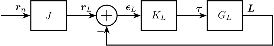
1.1 Control Schematic

\begin{tikzpicture}
  % Blocs
  \node[block] (J) at (0, 0) {$J$};
  \node[addb={+}{}{}{}{-}, right=1 of J] (subr) {};
  \node[block, right=0.8 of subr] (K) {$K_{L}$};
  \node[block, right=1 of K] (G) {$G_{L}$};

  % Connections and labels
  \draw[<-] (J.west)node[above left]{$\bm{r}_{n}$} -- ++(-1, 0);
  \draw[->] (J.east) -- (subr.west) node[above left]{$\bm{r}_{L}$};
  \draw[->] (subr.east) -- (K.west) node[above left]{$\bm{\epsilon}_{L}$};
  \draw[->] (K.east) -- (G.west) node[above left]{$\bm{\tau}$};
  \draw[->] (G.east) node[above right]{$\bm{L}$} -| ($(G.east)+(1, -1)$) -| (subr.south);
\end{tikzpicture}

1.2 Initialize the Stewart platform

stewart = initializeFramesPositions('H', 90e-3, 'MO_B', 45e-3);
% stewart = generateCubicConfiguration(stewart, 'Hc', 60e-3, 'FOc', 45e-3, 'FHa', 5e-3, 'MHb', 5e-3);
stewart = generateGeneralConfiguration(stewart);
stewart = computeJointsPose(stewart);
stewart = initializeStrutDynamics(stewart, 'Ki', 1e6*ones(6,1), 'Ci', 1e2*ones(6,1));
stewart = computeJacobian(stewart);

1.3 Initialize the Simulation

load('mat/conf_simscape.mat');

1.4 Identification of the plant

Let’s identify the transfer function from \(\bm{\tau}}\) to \(\bm{L}\).

%% Options for Linearized
options = linearizeOptions;
options.SampleTime = 0;

%% Name of the Simulink File
mdl = 'stewart_platform_control';

%% Input/Output definition
clear io; io_i = 1;
io(io_i) = linio([mdl, '/tau'], 1, 'openinput');  io_i = io_i + 1;
io(io_i) = linio([mdl, '/L'], 1, 'openoutput'); io_i = io_i + 1;

%% Run the linearization
G = linearize(mdl, io, options);
G.InputName  = {'F1', 'F2', 'F3', 'F4', 'F5', 'F6'};
G.OutputName = {'L1', 'L2', 'L3', 'L4', 'L5', 'L6'};

1.5 Plant Analysis

Diagonal terms Compare to off-diagonal terms

1.6 Controller Design

One integrator should be present in the controller.

A lead is added around the crossover frequency which is set to be around 500Hz.

% wint = 2*pi*100; % Integrate until [rad]
% wlead = 2*pi*500; % Location of the lead [rad]
% hlead = 2; % Lead strengh

% Kl = 1e6 * ... % Gain
%      (s + wint)/(s) * ... % Integrator until 100Hz
%      (1 + s/(wlead/hlead)/(1 + s/(wlead*hlead))); % Lead

wc = 2*pi*100;
Kl = 1/abs(freqresp(G(1,1), wc)) * wc/s * 1/(1 + s/(3*wc));
Kl = Kl * eye(6);