Cubic configuration for the Stewart Platform
Table of Contents
- 1. Configuration Analysis - Stiffness Matrix
- 1.1. Cubic Stewart platform centered with the cube center - Jacobian estimated at the cube center
- 1.2. Cubic Stewart platform centered with the cube center - Jacobian not estimated at the cube center
- 1.3. Cubic Stewart platform not centered with the cube center - Jacobian estimated at the cube center
- 1.4. Cubic Stewart platform not centered with the cube center - Jacobian estimated at the Stewart platform center
- 1.5. Conclusion
- 2. Configuration with the Cube’s center above the mobile platform
- 3. Cubic size analysis
- 4. Dynamic Coupling
- 5. Functions
The Cubic configuration for the Stewart platform was first proposed in geng94_six_degree_of_freed_activ. This configuration is quite specific in the sense that the active struts are arranged in a mutually orthogonal configuration connecting the corners of a cube. This configuration is now widely used (preumont07_six_axis_singl_stage_activ,jafari03_orthog_gough_stewar_platf_microm).
According to preumont07_six_axis_singl_stage_activ, the cubic configuration offers the following advantages:
This topology provides a uniform control capability and a uniform stiffness in all directions, and it minimizes the cross-coupling amongst actuators and sensors of different legs (being orthogonal to each other).
In this document, the cubic architecture is analyzed:
- In section 1, we study the link between the Stiffness matrix and the cubic architecture and we find what are the conditions to obtain a diagonal stiffness matrix
- In section 2, we study cubic configurations where the cube’s center is located above the mobile platform
- In section 3, we study the effect of the cube’s size on the Stewart platform properties
- In section 4, we study the dynamic coupling of the cubic configuration
To generate and study the Stewart platform with a Cubic configuration, the Matlab function generateCubicConfiguration is used (described here).
1 Configuration Analysis - Stiffness Matrix
First, we have to understand what is the physical meaning of the Stiffness matrix \(\bm{K}\).
The Stiffness matrix links forces \(\bm{f}\) and torques \(\bm{n}\) applied on the mobile platform at \(\{B\}\) to the displacement \(\Delta\bm{\mathcal{X}}\) of the mobile platform represented by \(\{B\}\) with respect to \(\{A\}\): \[ \bm{\mathcal{F}} = \bm{K} \Delta\bm{\mathcal{X}} \]
with:
- \(\bm{\mathcal{F}} = [\bm{f}\ \bm{n}]^{T}\)
- \(\Delta\bm{\mathcal{X}} = [\delta x, \delta y, \delta z, \delta \theta_{x}, \delta \theta_{y}, \delta \theta_{z}]^{T}\)
If the stiffness matrix is inversible, its inverse is the compliance matrix: \(\bm{C} = \bm{K}^{-1\) and: \[ \Delta \bm{\mathcal{X}} = C \bm{\mathcal{F}} \]
Thus, if the stiffness matrix is diagonal, the compliance matrix is also diagonal and a force (resp. torque) \(\bm{\mathcal{F}}_i\) applied on the mobile platform at \(\{B\}\) will induce a pure translation (resp. rotation) of the mobile platform represented by \(\{B\}\) with respect to \(\{A\}\).
One has to note that this is only valid in a static way.
We here study what makes the Stiffness matrix diagonal when using a cubic configuration.
1.1 Cubic Stewart platform centered with the cube center - Jacobian estimated at the cube center
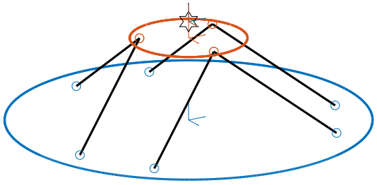
We create a cubic Stewart platform (figure 1) in such a way that the center of the cube (black dot) is located at the center of the Stewart platform (blue dot). The Jacobian matrix is estimated at the location of the center of the cube.
H = 100e-3;     % height of the Stewart platform [m]
MO_B = -H/2;     % Position {B} with respect to {M} [m]
Hc = H;         % Size of the useful part of the cube [m]
FOc = H + MO_B; % Center of the cube with respect to {F}
stewart = initializeStewartPlatform();
stewart = initializeFramesPositions(stewart, 'H', H, 'MO_B', MO_B);
stewart = generateCubicConfiguration(stewart, 'Hc', Hc, 'FOc', FOc, 'FHa', 0, 'MHb', 0);
stewart = computeJointsPose(stewart);
stewart = initializeStrutDynamics(stewart, 'K', ones(6,1));
stewart = computeJacobian(stewart);
stewart = initializeCylindricalPlatforms(stewart, 'Fpr', 175e-3, 'Mpr', 150e-3);
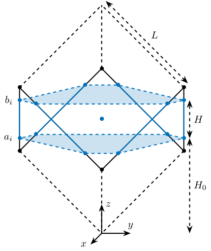
Figure 1: Centered cubic configuration
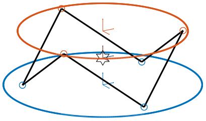
Figure 2: Cubic Stewart platform centered with the cube center - Jacobian estimated at the cube center (png, pdf)
| 2 | 0 | -2.5e-16 | 0 | 2.1e-17 | 0 |
| 0 | 2 | 0 | -7.8e-19 | 0 | 0 |
| -2.5e-16 | 0 | 2 | -2.4e-18 | -1.4e-17 | 0 |
| 0 | -7.8e-19 | -2.4e-18 | 0.015 | -4.3e-19 | 1.7e-18 |
| 1.8e-17 | 0 | -1.1e-17 | 0 | 0.015 | 0 |
| 6.6e-18 | -3.3e-18 | 0 | 1.7e-18 | 0 | 0.06 |
1.2 Cubic Stewart platform centered with the cube center - Jacobian not estimated at the cube center
We create a cubic Stewart platform with center of the cube located at the center of the Stewart platform (figure 1). The Jacobian matrix is not estimated at the location of the center of the cube.
H    = 100e-3; % height of the Stewart platform [m]
MO_B = 20e-3;  % Position {B} with respect to {M} [m]
Hc   = H;      % Size of the useful part of the cube [m]
FOc  = H/2;    % Center of the cube with respect to {F}
stewart = initializeStewartPlatform();
stewart = initializeFramesPositions(stewart, 'H', H, 'MO_B', MO_B);
stewart = generateCubicConfiguration(stewart, 'Hc', Hc, 'FOc', FOc, 'FHa', 0, 'MHb', 0);
stewart = computeJointsPose(stewart);
stewart = initializeStrutDynamics(stewart, 'K', ones(6,1));
stewart = computeJacobian(stewart);
stewart = initializeCylindricalPlatforms(stewart, 'Fpr', 175e-3, 'Mpr', 150e-3);

Figure 3: Cubic Stewart platform centered with the cube center - Jacobian not estimated at the cube center (png, pdf)
| 2 | 0 | -2.5e-16 | 0 | -0.14 | 0 |
| 0 | 2 | 0 | 0.14 | 0 | 0 |
| -2.5e-16 | 0 | 2 | -5.3e-19 | 0 | 0 |
| 0 | 0.14 | -5.3e-19 | 0.025 | 0 | 8.7e-19 |
| -0.14 | 0 | 2.6e-18 | 1.6e-19 | 0.025 | 0 |
| 6.6e-18 | -3.3e-18 | 0 | 8.9e-19 | 0 | 0.06 |
1.3 Cubic Stewart platform not centered with the cube center - Jacobian estimated at the cube center
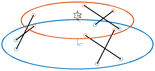
Here, the “center” of the Stewart platform is not at the cube center (figure 4). The Jacobian is estimated at the cube center.
H    = 80e-3; % height of the Stewart platform [m]
MO_B = -30e-3;  % Position {B} with respect to {M} [m]
Hc   = 100e-3;      % Size of the useful part of the cube [m]
FOc  = H + MO_B;    % Center of the cube with respect to {F}
stewart = initializeStewartPlatform();
stewart = initializeFramesPositions(stewart, 'H', H, 'MO_B', MO_B);
stewart = generateCubicConfiguration(stewart, 'Hc', Hc, 'FOc', FOc, 'FHa', 0, 'MHb', 0);
stewart = computeJointsPose(stewart);
stewart = initializeStrutDynamics(stewart, 'K', ones(6,1));
stewart = computeJacobian(stewart);
stewart = initializeCylindricalPlatforms(stewart, 'Fpr', 175e-3, 'Mpr', 150e-3);
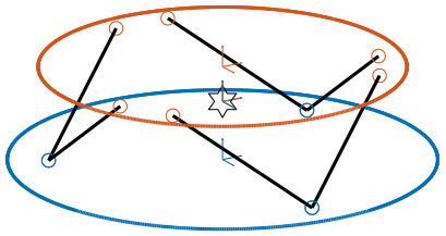
Figure 4: Cubic Stewart platform not centered with the cube center - Jacobian estimated at the cube center (png, pdf)
| 2 | 0 | -1.7e-16 | 0 | 4.9e-17 | 0 |
| 0 | 2 | 0 | -2.2e-17 | 0 | 2.8e-17 |
| -1.7e-16 | 0 | 2 | 1.1e-18 | -1.4e-17 | 1.4e-17 |
| 0 | -2.2e-17 | 1.1e-18 | 0.015 | 0 | 3.5e-18 |
| 4.4e-17 | 0 | -1.4e-17 | -5.7e-20 | 0.015 | -8.7e-19 |
| 6.6e-18 | 2.5e-17 | 0 | 3.5e-18 | -8.7e-19 | 0.06 |
We obtain \(k_x = k_y = k_z\) and \(k_{\theta_x} = k_{\theta_y}\), but the Stiffness matrix is not diagonal.
1.4 Cubic Stewart platform not centered with the cube center - Jacobian estimated at the Stewart platform center
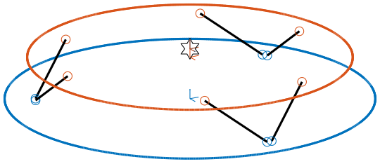
Here, the “center” of the Stewart platform is not at the cube center. The Jacobian is estimated at the center of the Stewart platform.
The center of the cube is at \(z = 110\). The Stewart platform is from \(z = H_0 = 75\) to \(z = H_0 + H_{tot} = 175\). The center height of the Stewart platform is then at \(z = \frac{175-75}{2} = 50\). The center of the cube from the top platform is at \(z = 110 - 175 = -65\).
H    = 100e-3; % height of the Stewart platform [m]
MO_B = -H/2;  % Position {B} with respect to {M} [m]
Hc   = 1.5*H;      % Size of the useful part of the cube [m]
FOc  = H/2 + 10e-3;    % Center of the cube with respect to {F}
stewart = initializeStewartPlatform();
stewart = initializeFramesPositions(stewart, 'H', H, 'MO_B', MO_B);
stewart = generateCubicConfiguration(stewart, 'Hc', Hc, 'FOc', FOc, 'FHa', 0, 'MHb', 0);
stewart = computeJointsPose(stewart);
stewart = initializeStrutDynamics(stewart, 'K', ones(6,1));
stewart = computeJacobian(stewart);
stewart = initializeCylindricalPlatforms(stewart, 'Fpr', 215e-3, 'Mpr', 195e-3);
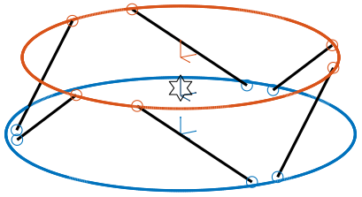
Figure 5: Cubic Stewart platform not centered with the cube center - Jacobian estimated at the Stewart platform center (png, pdf)
| 2 | 0 | 1.5e-16 | 0 | 0.02 | 0 |
| 0 | 2 | 0 | -0.02 | 0 | 0 |
| 1.5e-16 | 0 | 2 | -3e-18 | -2.8e-17 | 0 |
| 0 | -0.02 | -3e-18 | 0.034 | -8.7e-19 | 5.2e-18 |
| 0.02 | 0 | -2.2e-17 | -4.4e-19 | 0.034 | 0 |
| 5.9e-18 | -7.5e-18 | 0 | 3.5e-18 | 0 | 0.14 |
1.5 Conclusion
Here are the conclusion about the Stiffness matrix for the Cubic configuration:
- The cubic configuration permits to have \(k_x = k_y = k_z\) and \(k_{\theta_x} = k_{\theta_y}\)
- The stiffness matrix \(K\) is diagonal for the cubic configuration if the Jacobian is estimated at the cube center.
2 Configuration with the Cube’s center above the mobile platform
We saw in section 1 that in order to have a diagonal stiffness matrix, we need the cube’s center to be located at frames \(\{A\}\) and \(\{B\}\). Or, we usually want to have \(\{A\}\) and \(\{B\}\) located above the top platform where forces are applied and where displacements are expressed.
We here see if the cubic configuration can provide a diagonal stiffness matrix when \(\{A\}\) and \(\{B\}\) are above the mobile platform.
2.1 Having Cube’s center above the top platform
Let’s say we want to have a diagonal stiffness matrix when \(\{A\}\) and \(\{B\}\) are located above the top platform. Thus, we want the cube’s center to be located above the top center.
Let’s fix the Height of the Stewart platform and the position of frames \(\{A\}\) and \(\{B\}\):
H    = 100e-3; % height of the Stewart platform [m]
MO_B = 20e-3;  % Position {B} with respect to {M} [m]
We find the several Cubic configuration for the Stewart platform where the center of the cube is located at frame \(\{A\}\). The differences between the configuration are the cube’s size:
For each of the configuration, the Stiffness matrix is diagonal with \(k_x = k_y = k_y = 2k\) with \(k\) is the stiffness of each strut. However, the rotational stiffnesses are increasing with the cube’s size but the required size of the platform is also increasing, so there is a trade-off here.
Hc   = 0.4*H;    % Size of the useful part of the cube [m]
FOc  = H + MO_B; % Center of the cube with respect to {F}
| 2 | 0 | -2.8e-16 | 0 | 2.4e-17 | 0 |
| 0 | 2 | 0 | -2.3e-17 | 0 | 0 |
| -2.8e-16 | 0 | 2 | -2.1e-19 | 0 | 0 |
| 0 | -2.3e-17 | -2.1e-19 | 0.0024 | -5.4e-20 | 6.5e-19 |
| 2.4e-17 | 0 | 4.9e-19 | -2.3e-20 | 0.0024 | 0 |
| -1.2e-18 | 1.1e-18 | 0 | 6.2e-19 | 0 | 0.0096 |
Hc   = 1.5*H;    % Size of the useful part of the cube [m]
FOc  = H + MO_B; % Center of the cube with respect to {F}
| 2 | 0 | -1.9e-16 | 0 | 5.6e-17 | 0 |
| 0 | 2 | 0 | -7.6e-17 | 0 | 0 |
| -1.9e-16 | 0 | 2 | 2.5e-18 | 2.8e-17 | 0 |
| 0 | -7.6e-17 | 2.5e-18 | 0.034 | 8.7e-19 | 8.7e-18 |
| 5.7e-17 | 0 | 3.2e-17 | 2.9e-19 | 0.034 | 0 |
| -1e-18 | -1.3e-17 | 5.6e-17 | 8.4e-18 | 0 | 0.14 |
Hc   = 2.5*H;    % Size of the useful part of the cube [m]
FOc  = H + MO_B; % Center of the cube with respect to {F}
| 2 | 0 | -3e-16 | 0 | -8.3e-17 | 0 |
| 0 | 2 | 0 | -2.2e-17 | 0 | 5.6e-17 |
| -3e-16 | 0 | 2 | -9.3e-19 | -2.8e-17 | 0 |
| 0 | -2.2e-17 | -9.3e-19 | 0.094 | 0 | 2.1e-17 |
| -8e-17 | 0 | -3e-17 | -6.1e-19 | 0.094 | 0 |
| -6.2e-18 | 7.2e-17 | 5.6e-17 | 2.3e-17 | 0 | 0.37 |
2.2 Conclusion
We found that we can have a diagonal stiffness matrix using the cubic architecture when \(\{A\}\) and \(\{B\}\) are located above the top platform. Depending on the cube’s size, we obtain 3 different configurations.
3 Cubic size analysis
We here study the effect of the size of the cube used for the Stewart Cubic configuration.
We fix the height of the Stewart platform, the center of the cube is at the center of the Stewart platform and the frames \(\{A\}\) and \(\{B\}\) are also taken at the center of the cube.
We only vary the size of the cube.
3.1 Analysis
We initialize the wanted cube’s size.
Hcs = 1e-3*[250:20:350]; % Heights for the Cube [m]
Ks = zeros(6, 6, length(Hcs));
The height of the Stewart platform is fixed:
H = 100e-3; % height of the Stewart platform [m]
The frames \(\{A\}\) and \(\{B\}\) are positioned at the Stewart platform center as well as the cube’s center:
MO_B = -50e-3;  % Position {B} with respect to {M} [m]
FOc  = H + MO_B; % Center of the cube with respect to {F}
We find that for all the cube’s size, \(k_x = k_y = k_z = k\) where \(k\) is the strut stiffness. We also find that \(k_{\theta_x} = k_{\theta_y}\) and \(k_{\theta_z}\) are varying with the cube’s size (figure 9).
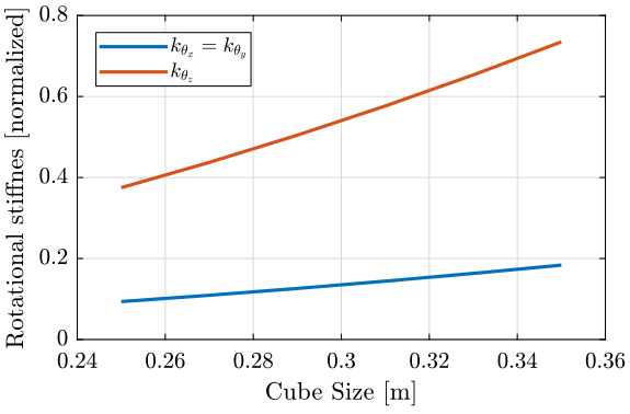
Figure 9: \(k_{\theta_x} = k_{\theta_y}\) and \(k_{\theta_z}\) function of the size of the cube
3.2 Conclusion
We observe that \(k_{\theta_x} = k_{\theta_y}\) and \(k_{\theta_z}\) increase linearly with the cube size.
In order to maximize the rotational stiffness of the Stewart platform, the size of the cube should be the highest possible.
4 Dynamic Coupling
4.1 Cube’s center at the Center of Mass of the Payload
4.2 Dynamic decoupling between the actuators and sensors
4.3 Conclusion
5 Functions
5.1 generateCubicConfiguration: Generate a Cubic Configuration
This Matlab function is accessible here.
Function description
function [stewart] = generateCubicConfiguration(stewart, args)
% generateCubicConfiguration - Generate a Cubic Configuration
%
% Syntax: [stewart] = generateCubicConfiguration(stewart, args)
%
% Inputs:
%    - stewart - A structure with the following fields
%        - geometry.H [1x1] - Total height of the platform [m]
%    - args - Can have the following fields:
%        - Hc  [1x1] - Height of the "useful" part of the cube [m]
%        - FOc [1x1] - Height of the center of the cube with respect to {F} [m]
%        - FHa [1x1] - Height of the plane joining the points ai with respect to the frame {F} [m]
%        - MHb [1x1] - Height of the plane joining the points bi with respect to the frame {M} [m]
%
% Outputs:
%    - stewart - updated Stewart structure with the added fields:
%        - platform_F.Fa  [3x6] - Its i'th column is the position vector of joint ai with respect to {F}
%        - platform_M.Mb  [3x6] - Its i'th column is the position vector of joint bi with respect to {M}
Documentation
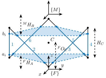
Figure 10: Cubic Configuration
Optional Parameters
arguments
    stewart
    args.Hc  (1,1) double {mustBeNumeric, mustBePositive} = 60e-3
    args.FOc (1,1) double {mustBeNumeric} = 50e-3
    args.FHa (1,1) double {mustBeNumeric, mustBeNonnegative} = 15e-3
    args.MHb (1,1) double {mustBeNumeric, mustBeNonnegative} = 15e-3
end
Check the stewart structure elements
assert(isfield(stewart.geometry, 'H'),   'stewart.geometry should have attribute H')
H = stewart.geometry.H;
Position of the Cube
We define the useful points of the cube with respect to the Cube’s center. \({}^{C}C\) are the 6 vertices of the cubes expressed in a frame {C} which is located at the center of the cube and aligned with {F} and {M}.
sx = [ 2; -1; -1];
sy = [ 0;  1; -1];
sz = [ 1;  1;  1];

R = [sx, sy, sz]./vecnorm([sx, sy, sz]);

L = args.Hc*sqrt(3);

Cc = R'*[[0;0;L],[L;0;L],[L;0;0],[L;L;0],[0;L;0],[0;L;L]] - [0;0;1.5*args.Hc];

CCf = [Cc(:,1), Cc(:,3), Cc(:,3), Cc(:,5), Cc(:,5), Cc(:,1)]; % CCf(:,i) corresponds to the bottom cube's vertice corresponding to the i'th leg
CCm = [Cc(:,2), Cc(:,2), Cc(:,4), Cc(:,4), Cc(:,6), Cc(:,6)]; % CCm(:,i) corresponds to the top cube's vertice corresponding to the i'th leg
Compute the pose
We can compute the vector of each leg \({}^{C}\hat{\bm{s}}_{i}\) (unit vector from \({}^{C}C_{f}\) to \({}^{C}C_{m}\)).
CSi = (CCm - CCf)./vecnorm(CCm - CCf);
We now which to compute the position of the joints \(a_{i}\) and \(b_{i}\).
Fa = CCf + [0; 0; args.FOc] + ((args.FHa-(args.FOc-args.Hc/2))./CSi(3,:)).*CSi;
Mb = CCf + [0; 0; args.FOc-H] + ((H-args.MHb-(args.FOc-args.Hc/2))./CSi(3,:)).*CSi;
Populate the stewart structure
stewart.platform_F.Fa = Fa;
stewart.platform_M.Mb = Mb;
Bibliography
- [geng94_six_degree_of_freed_activ] Geng & Haynes, Six Degree-Of-Freedom Active Vibration Control Using the Stewart Platforms, IEEE Transactions on Control Systems Technology, 2(1), 45-53 (1994). link. doi.
- [preumont07_six_axis_singl_stage_activ] Preumont, Horodinca, Romanescu, de Marneffe, Avraam, Deraemaeker, Bossens & Abu Hanieh, A Six-Axis Single-Stage Active Vibration Isolator Based on Stewart Platform, Journal of Sound and Vibration, 300(3-5), 644-661 (2007). link. doi.
- [jafari03_orthog_gough_stewar_platf_microm] Jafari & McInroy, Orthogonal Gough-Stewart Platforms for Micromanipulation, IEEE Transactions on Robotics and Automation, 19(4), 595-603 (2003). link. doi.