Sensor Fusion - Test Bench

1. Experimental Setup
2. Huddle Test
3. After identification
4. Sensor Dynamics

1 Experimental Setup

The goal of this experimental setup is to experimentally merge inertial sensors.

To merge the sensors, optimal and robust complementary filters are designed.

The inertial sensors used are shown in Table

Table 1: Inertial Sensors used
Type	Model
Accelerometer	PCB 393B05 - Vertical (link)
Geophone	Mark Product L-22 - Vertical

Table 2: Accelerometer (393B05) Specifications
Specification	Value
Sensitivity	1.02 [V/(m/s2)]
Resonant Frequency	> 2.5 [kHz]
Resolution (1 to 10kHz)	0.00004 [m/s2 rms]

Table 3: Geophone (L22) Specifications
Specification	Value
Sensitivity	To be measured [V/(m/s)]
Resonant Frequency	2 [Hz]

The ADC used are the IO131 Speedgoat module (link) with a 16bit resolution over +/- 10V.

The geophone signals are amplified using a DLPVA-100-B-D voltage amplified from Femto (link). The force sensor signal is amplified using a Low Noise Voltage Preamplifier from Ametek (link).

Geophone electronics:

gain: 10 (20dB)
low pass filter: 1.5Hz
hifh pass filter: 100kHz (2nd order)

Force Sensor electronics:

gain: 10 (20dB)
low pass filter: 1st order at 3Hz
high pass filter: 1st order at 30kHz

2 Huddle Test

The goal here is to measure the noise of the inertial sensors. Is also permits to measure the motion level when nothing is actuated.

2.1 Load Data

ht = load('./mat/huddle_test.mat', 'd', 'acc_1', 'acc_2', 'geo_1', 'geo_2', 'f_meas', 'u', 't');

2.2 Detrend Data

ht.d = detrend(ht.d, 0); % [m]
ht.acc_1 = detrend(ht.acc_1, 0); % [V]
ht.acc_2 = detrend(ht.acc_2, 0); % [V]
ht.geo_1 = detrend(ht.geo_1, 0); % [V]
ht.geo_2 = detrend(ht.geo_2, 0); % [V]
ht.f_meas = detrend(ht.f_meas, 0); % [V]

2.3 Compute PSD

We first define the parameters for the frequency domain analysis.

Ts = t(2) - t(1); % [s]
Fs = 1/Ts; % [Hz]

win = hanning(ceil(1*Fs));

Then we compute the Power Spectral Density using pwelch function.

[p_d,     f] = pwelch(ht.d, win, [], [], 1/Ts);
[p_acc1,  ~] = pwelch(ht.acc_1, win, [], [], 1/Ts);
[p_acc2,  ~] = pwelch(ht.acc_2, win, [], [], 1/Ts);
[p_geo1,  ~] = pwelch(ht.geo_1, win, [], [], 1/Ts);
[p_geo2,  ~] = pwelch(ht.geo_2, win, [], [], 1/Ts);
[p_fmeas, ~] = pwelch(ht.f_meas, win, [], [], 1/Ts);

2.4 Sensor Noise in Volts

[coh_acc, ~] = mscohere(ht.acc_1, ht.acc_2, win, [], [], Fs);
[coh_geo, ~] = mscohere(ht.geo_1, ht.geo_2, win, [], [], Fs);

pN_acc = p_acc1.*(1 - coh_acc);
pN_geo = p_geo1.*(1 - coh_geo);

PSD of the ADC quantization noise.

Sq = (20/2^16)^2/(12*Fs);

figure;
hold on;
plot(f, sqrt(pN_acc), '-', 'DisplayName', 'Accelerometers');
plot(f, sqrt(pN_geo), '-', 'DisplayName', 'Geophones');
plot(f, ones(size(f))*sqrt(Sq), '-', 'DisplayName', 'ADC');
hold off;
set(gca, 'xscale', 'log'); set(gca, 'yscale', 'log');
xlabel('Frequency [Hz]'); ylabel('ASD of the Measurement Noise $[V/\sqrt{Hz}]$');
xlim([1, 5000]);
legend('location', 'northeast');

3 After identification

3.1 Scale Data

Let’s use a model of the accelerometer and geophone to compute the motion from the measured voltage.

G_acc = 1/(1 + s/2/pi/2500); % [V/(m/s2)]

G_geo = 120*s^2/(s^2 + 2*0.7*2*pi*2*s + (2*pi*2)^2); % [V/(m/s)]

figure;
hold on;
set(gca, 'ColorOrderIndex', 1);
plot(f, sqrt(p_acc1)./abs(squeeze(freqresp(G_acc*s^2, f, 'Hz'))), ...
     'DisplayName', 'Accelerometer');
set(gca, 'ColorOrderIndex', 1);
plot(f, sqrt(p_acc2)./abs(squeeze(freqresp(G_acc*s^2, f, 'Hz'))), ...
     'HandleVisibility', 'off');
set(gca, 'ColorOrderIndex', 2);
plot(f, sqrt(p_geo1)./abs(squeeze(freqresp(G_geo*s, f, 'Hz'))), ...
     'DisplayName', 'Geophone');
set(gca, 'ColorOrderIndex', 2);
plot(f, sqrt(p_geo2)./abs(squeeze(freqresp(G_geo*s, f, 'Hz'))), ...
     'HandleVisibility', 'off');
set(gca, 'ColorOrderIndex', 3);
plot(f, sqrt(p_d), 'DisplayName', 'Interferometer');
hold off;
set(gca, 'Xscale', 'log'); set(gca, 'Yscale', 'log');
ylabel('ASD [$m/\sqrt{Hz}$]'); xlabel('Frequency [Hz]');
title('Huddle Test')
legend();

3.2 sdlkfj

acc_1 = lsim(inv(G_acc), ht.acc_1, ht.t);
acc_2 = lsim(inv(G_acc), ht.acc_2, ht.t);

geo_1 = lsim(inv(G_geo), ht.geo_1, ht.t);
geo_2 = lsim(inv(G_geo), ht.geo_2, ht.t);

3.3 Compare Time Domain Signals

figure;
hold on;
plot(t, acc_1);
plot(t, acc_2);
plot(t, geo_1);
plot(t, geo_2);
hold off;

3.4 Compute PSD

We first define the parameters for the frequency domain analysis.

Fs = 1/dt; % [Hz]

win = hanning(ceil(1*Fs));

Then we compute the Power Spectral Density using pwelch function.

[p_acc_1, f] = pwelch(acc_1, win, [], [], Fs);
[p_acc_2, ~] = pwelch(acc_2, win, [], [], Fs);
[p_geo_1, ~] = pwelch(geo_1, win, [], [], Fs);
[p_geo_2, ~] = pwelch(geo_2, win, [], [], Fs);

figure;
hold on;
plot(f, sqrt(p_acc_1));
plot(f, sqrt(p_acc_2));
hold off;
set(gca, 'xscale', 'log');
set(gca, 'yscale', 'log');
xlabel('Frequency [Hz]'); ylabel('ASD Accelerometers $\left[\frac{m/s}{\sqrt{Hz}}\right]$')
xlim([1, 5000]);

figure;
hold on;
plot(f, sqrt(p_geo_1));
plot(f, sqrt(p_geo_2));
hold off;
set(gca, 'xscale', 'log');
set(gca, 'yscale', 'log');
xlabel('Frequency [Hz]'); ylabel('ASD Geophones $\left[\frac{m/s}{\sqrt{Hz}}\right]$')
xlim([1, 5000]);

3.5 Dynamical Uncertainty

[T_acc, ~] = tfestimate(acc_1, acc_2, win, [], [], Fs);
[T_geo, ~] = tfestimate(geo_1, geo_2, win, [], [], Fs);

3.6 ADC Noise

Let’s note:

\(\Delta V\) the ADC range in [V]
\(n\) the number of bits
\(q = \frac{\Delta V}{2^n}\) the quantization in [V]
\(f_N\) the sampling frequency in [Hz]

The Power Spectral Density of the quantization noise is then:

\begin{equation} S_Q = \frac{q^2}{12 f_N} \quad [V^2/Hz] \end{equation}

Fs = 1/dt;
Sq = (20/2^16)^2/(12*Fs);

3.7 Sensor Noise

[coh_acc, ~] = mscohere(acc_1, acc_2, win, [], [], Fs);
[coh_geo, ~] = mscohere(geo_1, geo_2, win, [], [], Fs);

pN_acc = p_acc_1.*(1 - coh_acc);
pN_geo = p_geo_1.*(1 - coh_geo);

figure;
hold on;
plot(f, pN_acc, '-', 'DisplayName', 'Accelerometers');
plot(f, pN_geo, '-', 'DisplayName', 'Geophones');
hold off;
set(gca, 'xscale', 'log'); set(gca, 'yscale', 'log');
xlabel('Frequency [Hz]'); ylabel('ASD of the Measurement Noise $\left[\frac{m/s}{\sqrt{Hz}}\right]$');
xlim([1, 5000]);
legend('location', 'northeast');

4 Sensor Dynamics

Thanks to the interferometer, it is possible to compute the transfer function from the mass displacement to the voltage generated by the inertial sensors. This permits to estimate the sensor dynamics and to calibrate the sensors.

4.1 Load Data

ht = load('./mat/huddle_test.mat', 'd', 'acc_1', 'acc_2', 'geo_1', 'geo_2', 'f_meas', 'u', 't');
id_ol = load('./mat/identification_noise_bis.mat', 'd', 'acc_1', 'acc_2', 'geo_1', 'geo_2', 'f_meas', 'u', 't');

4.2 Time Domain Signals

Excitation signal: noise.

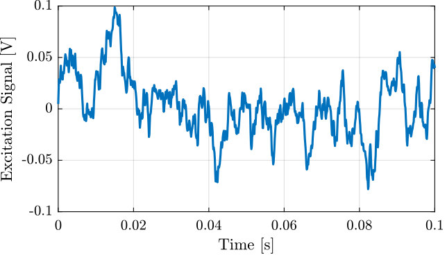
Figure 1: Excitation signal used for the first identification

4.3 Identification of the IFF Plant

4.3.1 Experimental Data

Ts = ht.t(2) - ht.t(1);
win = hann(ceil(10/Ts));

[tf_fmeas_est, f] = tfestimate(id_ol.u, id_ol.f_meas, win, [], [], 1/Ts); % [V/m]
[co_fmeas_est, ~] = mscohere(  id_ol.u, id_ol.f_meas, win, [], [], 1/Ts);

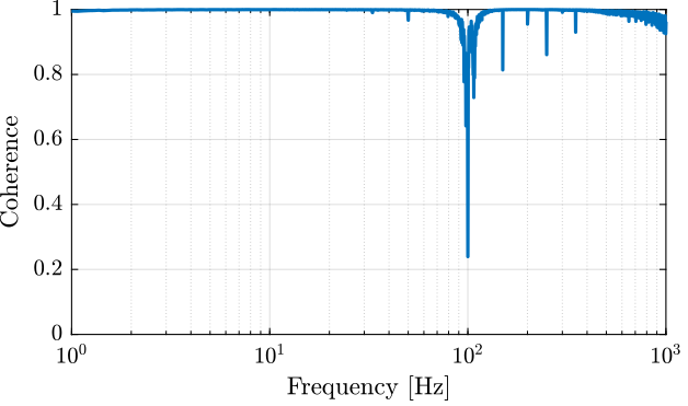
Figure 2: Coherence for the identification of the IFF plant

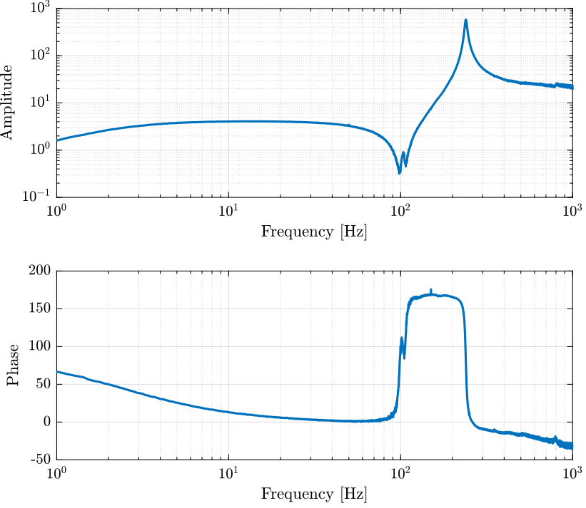
Figure 3: Bode plot of the identified IFF plant

4.3.2 Model of the IFF Plant

wz = 2*pi*102;
xi_z = 0.01;
wp = 2*pi*239.4;
xi_p = 0.015;

Giff = 2.2*(s^2 + 2*xi_z*s*wz + wz^2)/(s^2 + 2*xi_p*s*wp + wp^2) * ... % Dynamics
       10*(s/3/pi/(1 + s/3/pi)) * ... % Low pass filter and gain of the voltage amplifier
       exp(-Ts*s); % Time delay induced by ADC/DAC

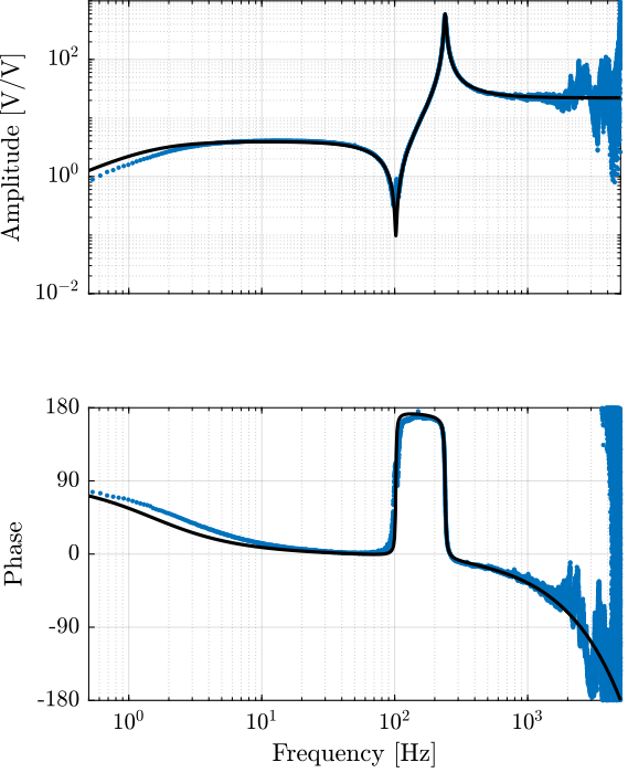
Figure 4: IFF Plant + Model

4.3.3 Root Locus and optimal Controller

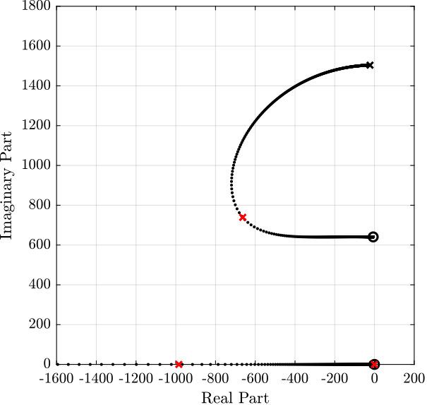
Figure 5: Root Locus for the IFF control

The controller that yield maximum damping is:

Kiff_opt = 102/(s + 2*pi*2);

4.4 Identification of Sensor Dynamics with IFF activated

4.4.1 Signals

A new identification is performed with the resonance damped. It helps to not induce too much motion at the resonance and damage the actuator.

id_cl = load('./mat/identification_noise_iff_bis.mat', 'd', 'acc_1', 'acc_2', 'geo_1', 'geo_2', 'f_meas', 'u', 't');

4.4.2 Verification of the achievable damping

[tf_G_ol_est, f] = tfestimate(id_ol.u, id_ol.d, win, [], [], 1/Ts);
[co_G_ol_est, ~] = mscohere(  id_ol.u, id_ol.d, win, [], [], 1/Ts);
[tf_G_cl_est, ~] = tfestimate(id_cl.u, id_cl.d, win, [], [], 1/Ts);
[co_G_cl_est, ~] = mscohere(  id_cl.u, id_cl.d, win, [], [], 1/Ts);

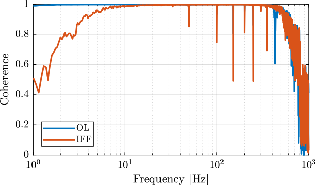
Figure 6: Coherence for the transfer function from F to d, with and without IFF

Don’t really understand the low frequency behavior.

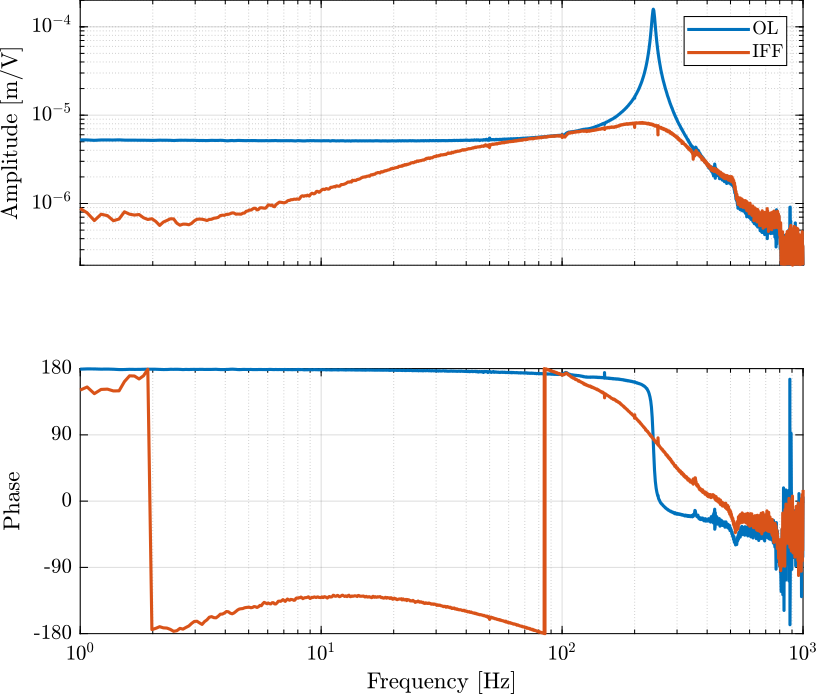
Figure 7: Coherence for the transfer function from F to d, with and without IFF

4.5 Generate the excitation signal

4.5.1 Requirements

The requirements on the excitation signal is:

General much larger motion that the measured motion during the huddle test
Don’t damage the actuator

To determine the perfect voltage signal to be generated, we need two things:

the transfer function from voltage to mass displacement
the PSD of the measured motion by the inertial sensors
not saturate the sensor signals
provide enough signal/noise ratio (good coherence) in the frequency band of interest (~0.5Hz to 3kHz)

4.5.2 Transfer function from excitation signal to displacement

Let’s first estimate the transfer function from the excitation signal in [V] to the generated displacement in [m] as measured by the inteferometer.

id_cl = load('./mat/identification_noise_iff_bis.mat', 'd', 'acc_1', 'acc_2', 'geo_1', 'geo_2', 'f_meas', 'u', 't');

win = hann(ceil(10/Ts));

[tf_G_cl_est, f] = tfestimate(id_cl.u, id_cl.d, win, [], [], 1/Ts);
[co_G_cl_est, ~] = mscohere(  id_cl.u, id_cl.d, win, [], [], 1/Ts);

Approximate transfer function from voltage output to generated displacement when IFF is used, in [m/V].

G_d_est = -5e-6*(2*pi*230)^2/(s^2 + 2*0.3*2*pi*240*s + (2*pi*240)^2);

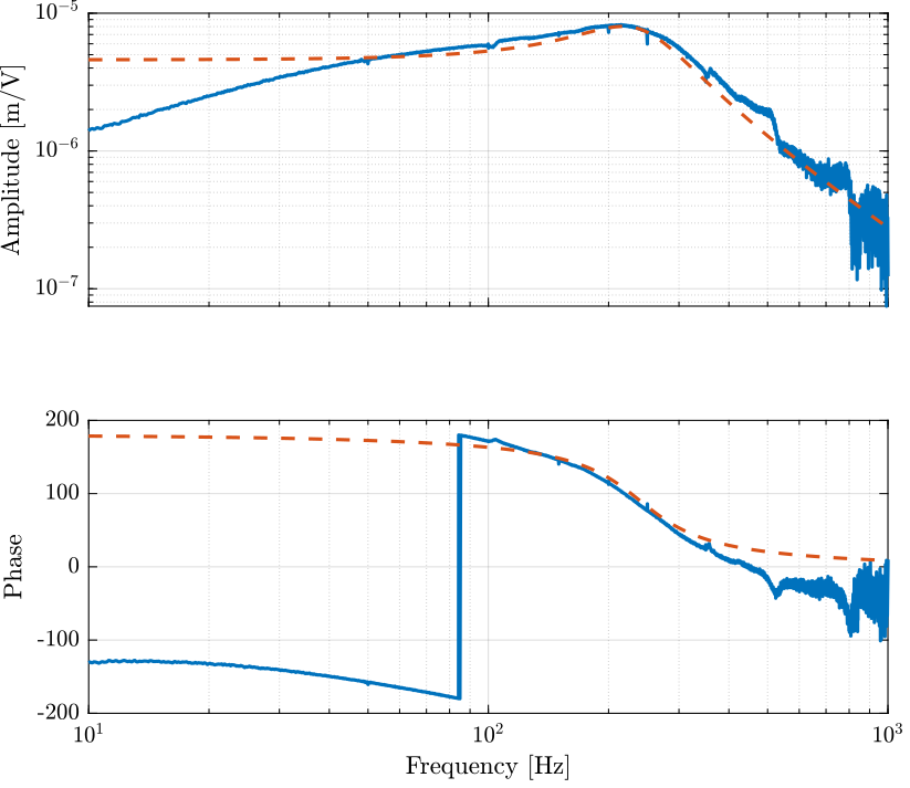
Figure 8: Estimation of the transfer function from the excitation signal to the generated displacement

4.5.3 Motion measured during Huddle test

We now compute the PSD of the measured motion by the inertial sensors during the huddle test.

ht = load('./mat/huddle_test.mat', 'd', 'acc_1', 'acc_2', 'geo_1', 'geo_2', 'f_meas', 'u', 't');

[p_d, f] = pwelch(ht.d, win, [], [], 1/Ts);
[p_acc1, ~] = pwelch(ht.acc_1, win, [], [], 1/Ts);
[p_acc2, ~] = pwelch(ht.acc_2, win, [], [], 1/Ts);
[p_geo1, ~] = pwelch(ht.geo_1, win, [], [], 1/Ts);
[p_geo2, ~] = pwelch(ht.geo_2, win, [], [], 1/Ts);

Using an estimated model of the sensor dynamics from the documentation of the sensors, we can compute the ASD of the motion in \(m/\sqrt{Hz}\) measured by the sensors.

G_acc = 1/(1 + s/2/pi/2500); % [V/(m/s2)]
G_geo = -120*s^2/(s^2 + 2*0.7*2*pi*2*s + (2*pi*2)^2); % [V/(m/s)]

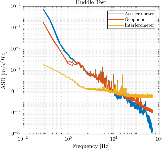
Figure 9: ASD of the motion measured by the sensors

From the ASD of the motion measured by the sensors, we can create an excitation signal that will generate much motion motion that the motion under no excitation.

We create G_exc that corresponds to the wanted generated motion.

G_exc = 0.2e-6/(1 + s/2/pi/2)/(1 + s/2/pi/50);

And we create a time domain signal y_d that have the spectral density described by G_exc.

Fs = 1/Ts;
t = 0:Ts:180; % Time Vector [s]
u = sqrt(Fs/2)*randn(length(t), 1); % Signal with an ASD equal to one

y_d = lsim(G_exc, u, t);

[pxx, ~] = pwelch(y_d, win, 0, [], Fs);

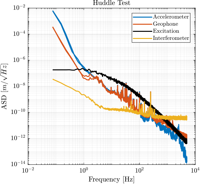
Figure 10: Comparison of the ASD of the motion during Huddle and the wanted generated motion

We can now generate the voltage signal that will generate the wanted motion.

y_v = lsim(G_exc * ... % from unit PSD to shaped PSD
           (1 + s/2/pi/50) * ... % Inverse of pre-filter included in the Simulink file
           1/G_d_est * ... % Wanted displacement => required voltage
           1/(1 + s/2/pi/5e3), ... %  Add some high frequency filtering
           u, t);

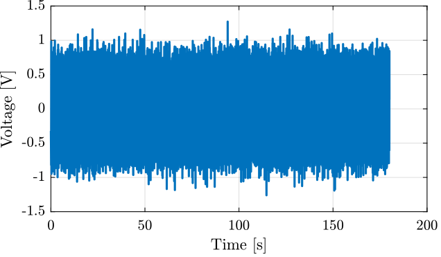
Figure 11: Generated excitation signal

4.6 Identification of the Inertial Sensors Dynamics

4.6.1 Load Data

id = load('./mat/identification_noise_opt_iff.mat', 'd', 'acc_1', 'acc_2', 'geo_1', 'geo_2', 'f_meas', 'u', 't');
ht = load('./mat/huddle_test.mat', 'd', 'acc_1', 'acc_2', 'geo_1', 'geo_2', 'f_meas', 'u', 't');

ht.d = detrend(ht.d, 0);
ht.acc_1 = detrend(ht.acc_1, 0);
ht.acc_2 = detrend(ht.acc_2, 0);
ht.geo_1 = detrend(ht.geo_1, 0);
ht.geo_2 = detrend(ht.geo_2, 0);
ht.f_meas = detrend(ht.f_meas, 0);

id.d = detrend(id.d, 0);
id.acc_1 = detrend(id.acc_1, 0);
id.acc_2 = detrend(id.acc_2, 0);
id.geo_1 = detrend(id.geo_1, 0);
id.geo_2 = detrend(id.geo_2, 0);
id.f_meas = detrend(id.f_meas, 0);

4.6.2 Compare PSD during Huddle and and during identification

Ts = ht.t(2) - ht.t(1);
win = hann(ceil(10/Ts));

[p_id_d, f] = pwelch(id.d, win, [], [], 1/Ts);
[p_id_acc1, ~] = pwelch(id.acc_1, win, [], [], 1/Ts);
[p_id_acc2, ~] = pwelch(id.acc_2, win, [], [], 1/Ts);
[p_id_geo1, ~] = pwelch(id.geo_1, win, [], [], 1/Ts);
[p_id_geo2, ~] = pwelch(id.geo_2, win, [], [], 1/Ts);
[p_id_fmeas, ~] = pwelch(id.f_meas, win, [], [], 1/Ts);

[p_ht_d, ~] = pwelch(ht.d, win, [], [], 1/Ts);
[p_ht_acc1, ~] = pwelch(ht.acc_1, win, [], [], 1/Ts);
[p_ht_acc2, ~] = pwelch(ht.acc_2, win, [], [], 1/Ts);
[p_ht_geo1, ~] = pwelch(ht.geo_1, win, [], [], 1/Ts);
[p_ht_geo2, ~] = pwelch(ht.geo_2, win, [], [], 1/Ts);
[p_ht_fmeas, ~] = pwelch(ht.f_meas, win, [], [], 1/Ts);

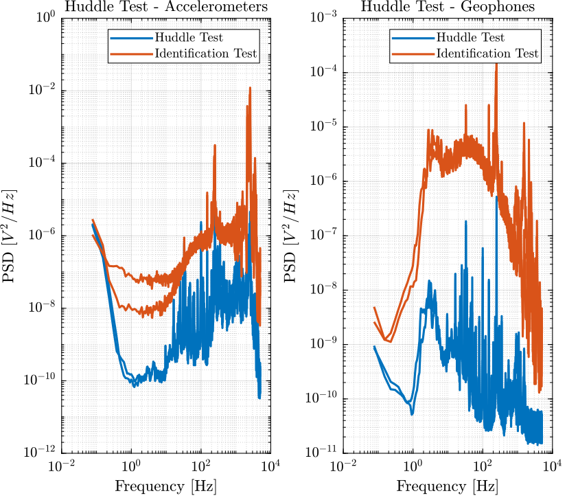
Figure 12: Comparison of the PSD of the measured motion during the Huddle test and during the identification

4.6.3 Compute transfer functions

[tf_acc1_est, f] = tfestimate(id.d, id.acc_1, win, [], [], 1/Ts);
[co_acc1_est, ~] = mscohere(  id.d, id.acc_1, win, [], [], 1/Ts);
[tf_acc2_est, ~] = tfestimate(id.d, id.acc_2, win, [], [], 1/Ts);
[co_acc2_est, ~] = mscohere(  id.d, id.acc_2, win, [], [], 1/Ts);

[tf_geo1_est, ~] = tfestimate(id.d, id.geo_1, win, [], [], 1/Ts);
[co_geo1_est, ~] = mscohere(  id.d, id.geo_1, win, [], [], 1/Ts);
[tf_geo2_est, ~] = tfestimate(id.d, id.geo_2, win, [], [], 1/Ts);
[co_geo2_est, ~] = mscohere(  id.d, id.geo_2, win, [], [], 1/Ts);

Figure 13: Coherence for the estimation of the sensor dynamics

Model of the inertial sensors:

G_acc = 1/(1 + s/2/pi/2500); % [V/(m/s2)]
G_geo = -1200*s^2/(s^2 + 2*0.7*2*pi*2*s + (2*pi*2)^2); % [[V/(m/s)]

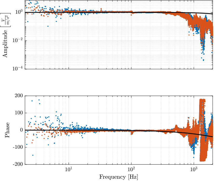
Figure 14: Identified dynamics of the accelerometers

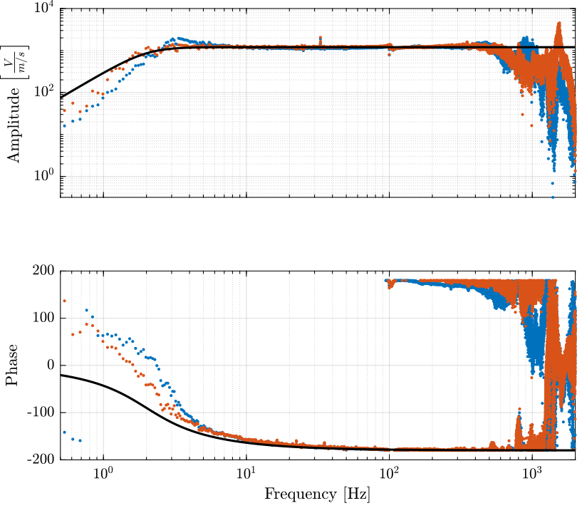
Figure 15: Identified dynamics of the geophones

4.7 Compare Time domain Estimation of the displacement

Let’s compare the measured accelerations instead of displacement (no integration).

G_lpf = 1/(1 + s/2/pi/5e3);

acc1_a = lsim(1/G_acc*G_lpf, id.acc_1, id.t);
acc2_a = lsim(1/G_acc*G_lpf, id.acc_2, id.t);

geo1_a = lsim(1/G_geo*s*G_lpf, id.geo_1, id.t);
geo2_a = lsim(1/G_geo*s*G_lpf, id.geo_2, id.t);

int_a = lsim(s^2*G_lpf*G_lpf, id.d, id.t);

figure;
hold on;
plot(id.t, int_a);
plot(id.t, acc1_a);
plot(id.t, acc2_a);
plot(id.t, geo1_a);
plot(id.t, geo2_a);
hold off;
xlabel('Time [s]'); ylabel('Acceleration [m]');