NASS - Uniaxial Model
Table of Contents
This report is also available as a pdf.
In this report, a uniaxial model of the Nano Active Stabilization System (NASS) is developed and used to have a first idea of the challenges involved in this complex system. Note that in this document, only the vertical direction is considered (which is the most stiff), but other directions were considered as well and yields similar conclusions. The model is schematically shown in Figure fig:uniaxial_overview_model_sections where the colors are representing the studied parts in different sections.
In order to have a relevant model, the micro-station dynamics is first identified and its model is tuned to match the measurements (Section sec:micro_station_model). Then, a model of the nano-hexapod is added on top of the micro-station. With added sample and sensors, this gives a uniaxial dynamical model of the NASS that will be used for further analysis (Section sec:nano_station_model).
The disturbances affecting the position accuracy are identified experimentally (Section sec:uniaxial_disturbances) and included in the model for dynamical noise budgeting (Section sec:uniaxial_noise_budgeting). In all the following analysis, there nano-hexapod stiffnesses are considered to better understand the trade-offs and to find the most adequate stiffness. Three sample masses are also considered to verify the robustness of the applied control strategies to a change of sample.
Three active damping techniques are then applied on the nano-hexapod. This helps to reduce the effect of disturbances as well as render the system easier to control afterwards (Section sec:uniaxial_active_damping).
Once the system is well damped, a feedback position controller is applied, and the obtained performances are compared (Section sec:uniaxial_position_control).
Conclusion remarks are given in Section sec:conclusion.
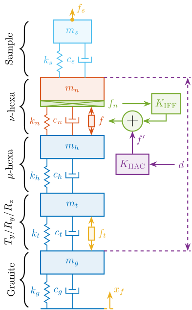
Figure 1: Uniaxial Micro-Station model in blue (Section sec:micro_station_model), Nano-Hexapod and sample models in red (Section sec:nano_station_model), Disturbances in yellow (Section sec:uniaxial_disturbances), Active Damping in green (Section sec:uniaxial_active_damping) and Position control in purple (Section sec:uniaxial_position_control)
1. Micro Station Model
In this section, a uni-axial model of the micro-station is tuned in order to match measurements made on the micro-station The measurement setup is shown in Figure fig:micro_station_first_meas_dynamics where several geophones are fixed to the micro-station and an instrumented hammer is used to inject forces on different stages of the micro-station.
From the measured frequency response functions (FRF), the model can be tuned to approximate the uniaxial dynamics of the micro-station.

Figure 2: Experimental Setup for the first dynamical measurements on the Micro-Station. Geophones are fixed to the micro-station, and the granite as well as the micro-hexapod’s top platform are impact with an instrumented hammer
1.1. Measured dynamics
The measurement setup is schematically shown in Figure fig:micro_station_meas_dynamics_schematic where:
- Two hammer hits are performed, one on the Granite (force \(F_g\)), and one on the micro-hexapod’s top platform (force \(F_h\))
- The inertial motion of the granite \(x_g\) and the micro-hexapod’s top platform \(x_h\) are measured using geophones.
From the forces applied by the instrumented hammer and the responses of the geophones, the following frequency response functions can be computed:
- from \(F_h\) to \(d_h\) (i.e. the compliance of the micro-station)
- from \(F_g\) to \(d_h\) (or from \(F_h\) to \(d_g\))
- from \(F_g\) to \(d_g\)

Figure 3: Measurement setup - Schematic
Due to the bad coherence at low frequency, the frequency response functions are only shown between 20 and 200Hz (Figure fig:uniaxial_measured_frf_vertical).
%% Load measured FRF
load('meas_microstation_frf.mat');

Figure 4: Measured Frequency Response Functions in the vertical direction
1.2. Uniaxial Model
The uni-axial model of the micro-station is shown in Figure fig:uniaxial_comp_frf_meas_model, with:
- Disturbances:
- \(x_f\): Floor motion
- \(f_t\): Stage vibrations
- Hammer impacts: \(F_h\) and \(F_g\).
- Geophones: \(x_h\) and \(x_g\)
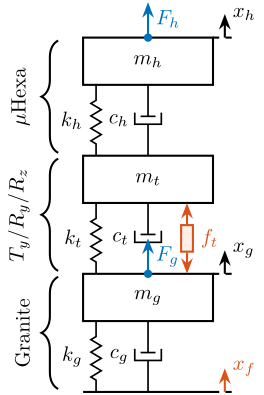
Figure 5: Uniaxial model of the micro-station
Masses are estimated from the CAD.
%% Parameters - Mass
mh = 15;   % Micro Hexapod [kg]
mt = 1200; % Ty + Ry + Rz [kg]
mg = 2500; % Granite [kg]
And stiffnesses from the data-sheet of stage manufacturers.
%% Parameters - Stiffnesses
kh = 6.11e+07; % [N/m]
kt = 5.19e+08; % [N/m]
kg = 9.50e+08; % [N/m]
The damping coefficients are tuned to match the identified damping from the measurements.
%% Parameters - damping
ch = 2*0.05*sqrt(kh*mh); % [N/(m/s)]
ct = 2*0.05*sqrt(kt*mt); % [N/(m/s)]
cg = 2*0.08*sqrt(kg*mg); % [N/(m/s)]
1.3. Comparison of the model and measurements
The comparison between the measurements and the model is done in Figure fig:uniaxial_comp_frf_meas_model.
As the model is simplistic, the goal is not to match exactly the measurement but to have a first approximation. More accurate models will be used later on.
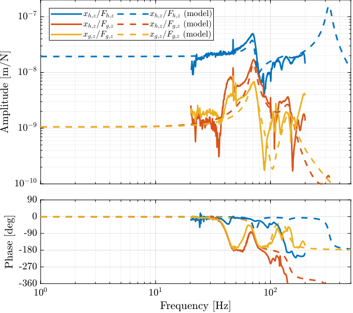
Figure 6: Comparison of the measured FRF and identified ones from the uni-axial model
2. Nano-Hexapod Model
A model of the nano-hexapod and sample is now added on top of the uni-axial model of the micro-station (Figure fig:uniaxial_model_micro_station-nass).
Disturbances (shown in red) are:
- \(f_s\): direct forces applied to the sample (for instance cable forces)
- \(f_t\): disturbances coming from the imperfect stage scanning performances
- \(x_f\): floor motion
The control signal is the force applied by the nano-hexapod \(f\) and the measurement is the relative motion between the sample and the granite \(d\).
The sample is here considered as a rigid body and rigidly fixed to the nano-hexapod. The effect of having resonances between the sample’s point of interest and the nano-hexapod actuator will be considered in further analysis.
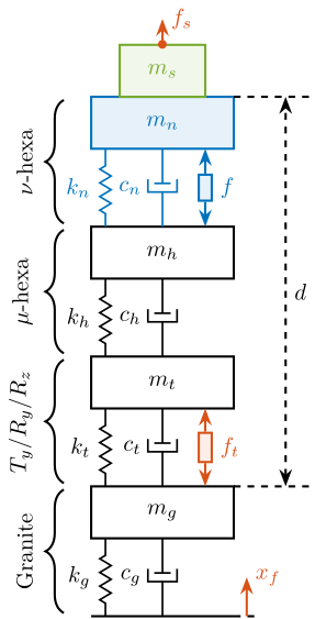
Figure 7: Uni-axial model of the micro-station with added nano-hexapod (represented in blue) and sample (represented in green)
2.1. Nano-Hexapod Parameters
The parameters for the nano-hexapod and sample are:
- \(m_s\) the sample mass that can vary from 1kg up to 50kg
- \(m_n\) the nano-hexapod mass which is set to 15kg
- \(k_n\) the nano-hexapod stiffness, which can vary depending on the chosen architecture/technology
As a first example, let’s choose a nano-hexapod stiffness of \(10\,N/\mu m\) and a sample mass of 10kg.
%% Nano-Hexapod Parameters
mn = 15; % [kg]
kn = 1e7; % [N/m]
cn = 2*0.01*sqrt(mn*kn); % [N/(m/s)]

%% Sample Mass
ms = 10; % [kg]
2.2. Obtained Dynamics
The sensitivity to disturbances (i.e. \(x_f\), \(f_t\) and \(f_s\)) are shown in Figure fig:uniaxial_sensitivity_dist_first_params. The plant (i.e. the transfer function from actuator force \(f\) to measured displacement \(d\)) is shown in Figure fig:uniaxial_plant_first_params.
For further analysis, 9 configurations are considered: three nano-hexapod stiffnesses (\(k_n = 0.01\,N/\mu m\), \(k_n = 1\,N/\mu m\) and \(k_n = 100\,N/\mu m\)) combined with three sample’s masses (\(m_s = 1\,kg\), \(m_s = 25\,kg\) and \(m_s = 50\,kg\)).

Figure 8: Sensitivity to disturbances
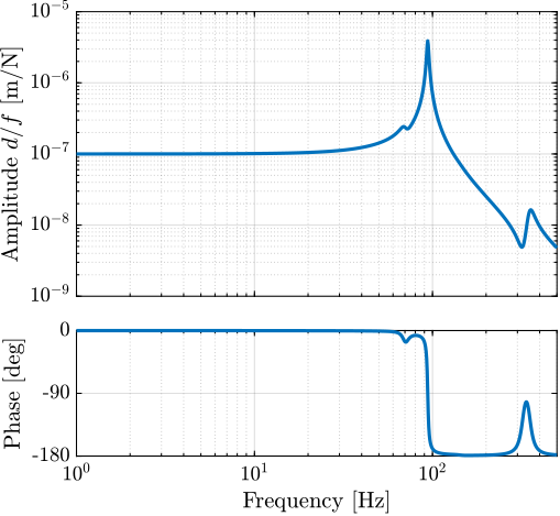
Figure 9: Bode Plot of the transfer function from actuator forces to measured displacement by the metrology
3. Disturbance Identification
In order to measure disturbances, two geophones are used, on located on the floor and on on the micro-hexapod’s top platform (see Figure fig:micro_station_meas_disturbances).
The geophone on the floor is used to measured the floor motion \(x_f\) while the geophone on the micro-hexapod is used to measure vibrations introduced by scanning of the \(T_y\) stage and \(R_z\) stage.

Figure 10: Disturbance measurement setup - Schematic

Figure 11: Two geophones are used to measure the micro-station vibrations induced by the scanning of the \(T_y\) and \(R_z\) stages
3.1. Ground Motion
The geophone fixed to the floor to measure the floor motion.
%% Load floor motion data
% t: time in [s]
% V: measured voltage genrated by the geophone and amplified by a 60dB gain voltage amplifier [V]
load('ground_motion_measurement.mat', 't', 'V');
The voltage generated by each geophone is amplified using a voltage amplifier (gain of 60dB) before going to the ADC. The sensitivity of the geophone as well as the gain of the voltage amplifier are then taken into account to reconstruct the floor displacement.
%% Sensitivity of the geophone
S0 = 88; % Sensitivity [V/(m/s)]
f0 = 2; % Cut-off frequency [Hz]

S = S0*(s/2/pi/f0)/(1+s/2/pi/f0); % Geophone's transfer function [V/(m/s)]

%% Gain of the voltage amplifier
G0_db = 60; % [dB]
G0 = 10^(G0_db/20); % [abs]

%% Transfer function from measured voltage to displacement
G_geo = 1/S/G0/s; % [m/V]
The PSD \(S_{V_f}\) of the measured voltage \(V_f\) is computed.
%% Compute measured voltage PSD
Fs = 1/(t(2)-t(1)); % Sampling Frequency [Hz]
win = hanning(ceil(2*Fs)); % Hanning window

[psd_V, f] = pwelch(V, win, [], [], Fs); % [V^2/Hz]
The PSD of the corresponding displacement can be computed as follows:
\begin{equation} S_{x_f}(\omega) = \frac{S_{V_f}(\omega)}{|S_{\text{geo}}(j\omega)| \cdot G_{\text{amp}} \cdot \omega} \end{equation}with:
- \(S_{\text{geo}}\) the sensitivity of the Geophone in \([Vs/m]\)
- \(G_{\text{amp}}\) the gain of the voltage amplifier
- \(\omega\) is here to integrate and have the displacement instead of the velocity
%% Ground Motion ASD
psd_xf = psd_V.*abs(squeeze(freqresp(G_geo, f, 'Hz'))).^2; % [m^2/Hz]
The amplitude spectral density \(\Gamma_{x_f}\) of the measured displacement \(x_f\) is shown in Figure fig:asd_floor_motion_id31.

Figure 12: Measured Amplitude Spectral Density of the Floor motion on ID31
3.2. Stage Vibration
During Spindle rotation (here at 6rpm), the granite velocity and micro-hexapod’s top platform velocity are measured with the geophones.
%% Measured velocity of granite and hexapod during spindle rotation
% t: time in [s]
% vg: measured granite velocity [m/s]
% vg: measured micro-hexapod's top platform velocity [m/s]
load('meas_spindle_on.mat', 't', 'vg', 'vh');
spindle_off = load('meas_spindle_off.mat', 't', 'vg', 'vh'); % No Rotation
The Power Spectral Density of the relative velocity between the hexapod and the granite is computed.
%% Compute Power Spectral Density of the relative velocity between granite and hexapod during spindle rotation
Fs = 1/(t(2)-t(1)); % Sampling Frequency [Hz]
win = hanning(ceil(2*Fs)); % Hanning window

[psd_vft, f] = pwelch(vh-vg, win, [], [], Fs); % [(m/s)^2/Hz]
[psd_off, ~] = pwelch(spindle_off.vh-spindle_off.vg, win, [], [], Fs); % [(m/s)^2/Hz]
It is then integrated to obtain the Amplitude Spectral Density of the relative motion which is compared with a non-rotating case (Figure fig:asd_vibration_spindle_rotation). It is shown that the spindle rotation induces vibrations in a wide frequency spectrum.

Figure 13: Measured Amplitude Spectral Density of the relative motion between the granite and the micro-hexapod’s top platform during Spindle rotating
In order to compute the equivalent disturbance force \(f_t\) that induces such motion, the transfer function from \(f_t\) to the relative motion of the hexapod’s top platform and the granite is extracted from the model. The power spectral density \(\Gamma_{f_{t}}\) of the disturbance force can be computed as follows:
\begin{equation} \Gamma_{f_{t}}(\omega) = \frac{\Gamma_{v_{t}}(\omega)}{|G_{\text{model}}(j\omega)|^2} \end{equation}with:
- \(\Gamma_{v_{t}}\) the measured power spectral density of the relative motion between the micro-hexapod’s top platform and the granite during the spindle’s rotation
- \(G_{\text{model}}\) the transfer function (extracted from the uniaxial model) from \(f_t\) to the relative motion between the micro-hexapod’s top platform and the granite
The obtained amplitude spectral density of the disturbance force \(f_t\) is shown in Figure fig:asd_disturbance_force.

Figure 14: Estimated disturbance force ft from measurement and uniaxial model
The vibrations induced by the \(T_y\) stage are not considered here as:
- the induced vibrations have less amplitude than the vibrations induced by the \(R_z\) stage
- it can be scanned at lower velocities if the induced vibrations are an issue
4. Open-Loop Dynamic Noise Budgeting
Now that we have a model of the NASS and an estimation of the power spectral density of the disturbances, it is possible to perform an open-loop dynamic noise budgeting.
4.1. Sensitivity to disturbances
From the Uni-axial model, the transfer function from the disturbances (\(f_s\), \(x_f\) and \(f_t\)) to the displacement \(d\) are computed.
This is done for two extreme sample masses \(m_s = 1\,\text{kg}\) and \(m_s = 50\,\text{kg}\) and three nano-hexapod stiffnesses:
- \(k_n = 0.01\,N/\mu m\) that could represent a voice coil actuator with soft flexible guiding
- \(k_n = 1\,N/\mu m\) that could represent a voice coil actuator with a stiff flexible guiding or a mechanically amplified piezoelectric actuator
- \(k_n = 100\,N/\mu m\) that could represent a stiff piezoelectric stack actuator
The obtained sensitivity to disturbances for the three nano-hexapod stiffnesses are shown in Figure fig:uniaxial_sensitivity_disturbances_nano_hexapod_stiffnesses for the light sample (same conclusions can be drawn with the heavy one).
From Figure fig:uniaxial_sensitivity_disturbances_nano_hexapod_stiffnesses, following can be concluded for the soft nano-hexapod:
- It is more sensitive to forces applied on the sample (cable forces for instance), which is expected due to the lower stiffness
- Between the suspension mode of the nano-hexapod (here at 5Hz) and the first mode of the micro-station (here at 70Hz), the disturbances induced by the stage vibrations are filtered out.
- Above the suspension mode of the nano-hexapod, the sample’s motion is unaffected by the floor motion, and therefore the sensitivity to floor motion is almost \(1\).

Figure 15: Sensitivity to disturbances for three different nano-hexpod stiffnesses
4.2. Open-Loop Dynamic Noise Budgeting
Now, the power spectral density of the disturbances is taken into account to estimate the residual motion \(d\) in each case.
The Cumulative Amplitude Spectrum of the relative motion \(d\) due to both the floor motion \(x_f\) and the stage vibrations \(f_t\) are shown in Figure fig:uniaxial_cas_d_disturbances_stiffnesses for the three nano-hexapod stiffnesses.
It is shown that the effect of the floor motion is much less than the stage vibrations, except for the soft nano-hexapod below 5Hz.
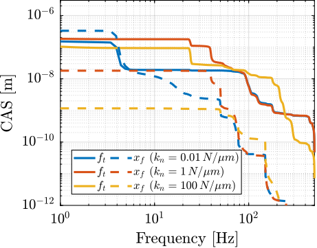
Figure 16: Cumulative Amplitude Spectrum of the relative motion d, due to both the floor motion and the stage vibrations (light sample)
The total cumulative amplitude spectrum for the three nano-hexapod stiffnesses and for the two sample’s masses are shown in Figure fig:uniaxial_cas_d_disturbances_payload_masses. The conclusion is that the sample’s mass has little effect on the cumulative amplitude spectrum of the relative motion \(d\).
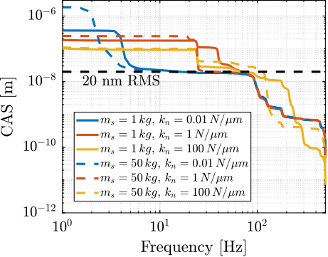
Figure 17: Cumulative Amplitude Spectrum of the relative motion d due to all disturbances, for two sample masses
4.3. Conclusion
The conclusion is that in order to have a closed-loop residual vibration \(d \approx 20\,nm\text{ rms}\), if a simple feedback controller is used, the required closed-loop bandwidth would be:
- \(\approx 10\,\text{Hz}\) for the soft nano-hexapod (\(k_n = 0.01\,N/\mu m\))
- \(\approx 50\,\text{Hz}\) for the relatively stiff nano-hexapod (\(k_n = 1\,N/\mu m\))
- \(\approx 100\,\text{Hz}\) for the stiff nano-hexapod (\(k_n = 100\,N/\mu m\))
This can be explain by the fact that above the suspension mode of the nano-hexapod, the stage vibrations are filtered out (see Figure fig:uniaxial_sensitivity_disturbances_nano_hexapod_stiffnesses).
This gives a first advantage to having a soft nano-hexapod.
5. Active Damping
In this section, three active damping are applied on the nano-hexapod (see Figure fig:uniaxial_active_damping_strategies): Integral Force Feedback (IFF), Relative Damping Control (RDC) and Direct Velocity Feedback (DVF).
These active damping techniques are compared in terms of:
- Reduction of the effect of disturbances (i.e. \(x_f\), \(f_t\) and \(f_s\)) on the displacement \(d\)
- Achievable damping
- Robustness to a change of sample’s mass

Figure 18: Three active damping strategies: Integral Force Feedback (IFF) using a force sensor, Relative Damping Control (RDC) using a relative displacement sensor, and Direct Velocity Feedback (DVF) using a geophone
5.1. Active Damping Strategies
The Integral Force Feedback strategy consists of using a force sensor in series with the actuator (see Figure fig:uniaxial_active_damping_iff_equiv, left).
The control strategy consists of integrating the measured force and feeding it back to the actuator:
\begin{equation} K_{\text{IFF}}(s) = \frac{g}{s} \end{equation}The mechanical equivalent of this strategy is to add a dashpot in series with the actuator stiffness with a damping coefficient equal to the stiffness of the actuator divided by the controller gain \(k/g\) (see Figure fig:uniaxial_active_damping_iff_equiv, right).
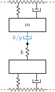
Figure 19: Integral Force Feedback is equivalent as to add a damper in series with the stiffness (the initial damping is here neglected for simplicity)
For the Relative Damping Control strategy, a relative motion sensor that measures the motion of the actuator is used (see Figure fig:uniaxial_active_damping_rdc_equiv, left).
The derivative of this relative motion is used for the feedback signal:
\begin{equation} K_{\text{RDC}}(s) = - g \cdot s \end{equation}The mechanical equivalent is to add a dashpot in parallel with the actuator with a damping coefficient equal to the controller gain \(g\) (see Figure fig:uniaxial_active_damping_rdc_equiv, right).
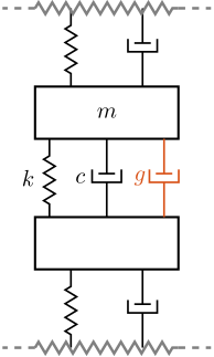
Figure 20: Relative Damping Control is equivalent as adding a damper in parallel with the actuator/relative motion sensor
Finally, the Direct Velocity Feedback strategy consists of using an inertial sensor (usually a geophone), that measured the “absolute” velocity of the body fixed on top of the actuator (se Figure fig:uniaxial_active_damping_dvf_equiv, left).
The measured velocity is then fed back to the actuator:
\begin{equation} K_{\text{DVF}}(s) = - g \end{equation}This is equivalent as to fix a dashpot (with a damping coefficient equal to the controller gain \(g\)) between the body (one which the inertial sensor is fixed) and an inertial reference frame (see Figure fig:uniaxial_active_damping_dvf_equiv, right). This is usually refers to as “sky hook damper”.
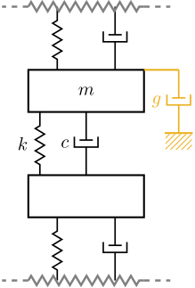
Figure 21: Direct velocity Feedback using an inertial sensor is equivalent to a “sky hook damper”
5.2. Plant Dynamics for Active Damping
The plant dynamics for all three active damping techniques are shown in Figure fig:uniaxial_plant_active_damping_techniques. All have alternating poles and zeros meaning that the phase is bounded to \(\pm 90\,\text{deg}\) which makes the controller very robust.
When the nano-hexapod’s suspension modes are at lower frequencies than the resonances of the micro-station (blue and red curves in Figure fig:uniaxial_plant_active_damping_techniques), the resonances of the micro-stations have little impact on the transfer functions from IFF and DVF.
For the stiff nano-hexapod, the micro-station dynamics can be seen on the transfer functions in Figure fig:uniaxial_plant_active_damping_techniques. Therefore, it is expected that the micro-station dynamics might impact the achievable damping if a stiff nano-hexapod is used.

Figure 22: Plant dynamics for the three active damping techniques (IFF: right, RDC: middle, DVF: left), for three nano-hexapod stiffnesses (\(k_n = 0.01\,N/\mu m\) in blue, \(k_n = 1\,N/\mu m\) in red and \(k_n = 100\,N/\mu m\) in yellow) and three sample’s masses (\(m_s = 1\,kg\): solid curves, \(m_s = 25\,kg\): dot-dashed curves, and \(m_s = 50\,kg\): dashed curves).
5.3. Achievable Damping - Root Locus
The Root Locus are computed for the three nano-hexapod stiffnesses and for the three active damping techniques. They are shown in Figure fig:uniaxial_root_locus_damping_techniques.
All three active damping approach can lead to critical damping of the nano-hexapod suspension mode.
There is even a little bit of authority on micro-station modes with IFF and DVF applied on the stiff nano-hexapod (Figure fig:uniaxial_root_locus_damping_techniques, right) and with RDC for a soft nano-hexapod (Figure fig:uniaxial_root_locus_damping_techniques_micro_station_mode). This can be explained by the fact that above the suspension mode of the soft nano-hexapod, the relative motion sensor acts as an inertial sensor for the micro-station top platform. Therefore, it is like DVF was applied (the nano-hexapod acts as a geophone!).

Figure 23: Root Loci for the three active damping techniques (IFF in blue, RDC in red and DVF in yellow). This is shown for three nano-hexapod stiffnesses.
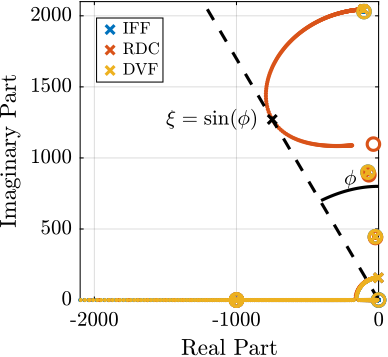
Figure 24: Root Locus for the three damping techniques. It is shown that the RDC active damping technique has some authority on one mode of the micro-station. This mode corresponds to the suspension mode of the micro-hexapod.
5.4. Change of sensitivity to disturbances
The sensitivity to disturbances (direct forces \(f_s\), stage vibrations \(f_t\) and floor motion \(x_f\)) for all three active damping techniques are compared in Figure fig:uniaxial_sensitivity_dist_active_damping. The comparison is done with the nano-hexapod having a stiffness \(k_n = 1\,N/\mu m\).
Conclusions from Figure fig:uniaxial_sensitivity_dist_active_damping are:
- IFF degrades the sensitivity to direct forces on the sample (i.e. the compliance) below the resonance of the nano-hexapod
- RDC degrades the sensitivity to stage vibrations around the nano-hexapod’s resonance as compared to the other two methods
- both IFF and DVF degrades the sensitivity to floor motion below the resonance of the nano-hexapod

Figure 25: Change of sensitivity to disturbance with all three active damping strategies
5.5. Noise Budgeting after Active Damping
Cumulative Amplitude Spectrum of the distance \(d\) with all three active damping techniques are compared in Figure fig:uniaxial_cas_active_damping. All three active damping methods are giving similar results (except the RDC which is a little bit worse for the stiff nano-hexapod).
Compare to the open-loop case, the active damping helps to lower the vibrations induced by the nano-hexapod resonance.

Figure 26: Comparison of the cumulative amplitude spectrum (CAS) of the distance \(d\) for all three active damping techniques (OL in black, IFF in blue, RDC in red and DVF in yellow).
5.6. Obtained Damped Plant
The transfer functions from the plant input \(f\) to the relative displacement \(d\) while the active damping is implemented are shown in Figure fig:uniaxial_damped_plant_three_active_damping_techniques. All three active damping techniques yield similar damped plants.

Figure 27: Obtained damped transfer function from f to d for the three damping techniques
The damped plants are shown in Figure fig:uniaxial_damped_plant_change_sample_mass for all three techniques, with the three considered nano-hexapod stiffnesses and sample’s masses.

Figure 28: Damped plant \(d/f\) - Robustness to change of sample’s mass for all three active damping techniques. Grey curves are the open-loop (i.e. undamped) plants.
5.7. Robustness to change of payload’s mass
The Root Locus for the three damping techniques are shown in Figure fig:uniaxial_active_damping_robustness_mass_root_locus for three sample’s mass (1kg, 25kg and 50kg). The closed-loop poles are shown by the squares for a specific gain.
We can see that having heavier samples yields larger damping for IFF and smaller damping for RDC and DVF.

Figure 29: Active Damping Robustness to change of sample’s mass - Root Locus for all three damping techniques with 3 different sample’s masses
5.8. Conclusion
Conclusions for Active Damping:
- All three active damping techniques yields good damping (Figure fig:uniaxial_root_locus_damping_techniques) and similar remaining vibrations (Figure fig:uniaxial_cas_active_damping)
- The obtained damped plants (Figure fig:uniaxial_damped_plant_change_sample_mass) are equivalent for the three active damping techniques
- Which one to be used will be determined with the use of more accurate models and will depend on which is the easiest to implement in practice
| IFF | RDC | DVF | |
|---|---|---|---|
| Sensor | Force sensor | Relative motion sensor | Inertial sensor |
| Damping | Up to critical | Up to critical | Up to Critical |
| Robustness | Requires collocation | Requires collocation | Impacted by geophone resonances |
| \(f_s\) Disturbance | \(\nearrow\) at low frequency | \(\searrow\) near resonance | \(\searrow\) near resonance |
| \(f_t\) Disturbance | \(\searrow\) near resonance | \(\nearrow\) near resonance | \(\searrow\) near resonance |
| \(x_f\) Disturbance | \(\nearrow\) at low frequency | \(\searrow\) near resonance | \(\nearrow\) at low frequency |
6. Position Feedback Controller
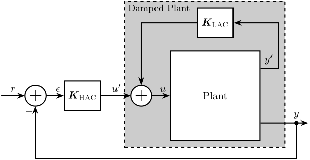
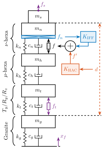
The High Authority Control - Low Authority Control (HAC-LAC) architecture is shown in Figure fig:uniaxial_hac_lac_architecture. It corresponds to a two step control strategy:
- First, an active damping controller \(\bm{K}_{\textsc{LAC}}\) is implemented (see Section sec:uniaxial_active_damping). It allows to reduce the vibration level, and it also makes the damped plant (transfer function from \(u^{\prime}\) to \(y\)) easier to control than the undamped plant (transfer function from \(u\) to \(y\)).
- Then, a position controller \(\bm{K}_{\textsc{HAC}}\) is implemented.
Combined with the uniaxial model, it is shown in Figure fig:uniaxial_hac_lac_model.
6.1. Damped Plant Dynamics
As was shown in Section sec:uniaxial_active_damping, all three proposed active damping techniques yield similar damping plants. Therefore, Integral Force Feedback will be used in this section to study the HAC-LAC performances.
The obtained damped plants for the three nano-hexapod stiffnesses are shown in Figure fig:uniaxial_hac_iff_damped_plants_masses.

Figure 30: Obtained damped plant using Integral Force Feedback for three sample’s masses
6.2. Position Feedback Controller
The objective now is to design a position feedback controller for each of the three nano-hexapods that are robust to the change of sample’s mass.
The required feedback bandwidth was approximately determined un Section sec:uniaxial_noise_budgeting:
- \(\approx 10\,\text{Hz}\) for the soft nano-hexapod (\(k_n = 0.01\,N/\mu m\)). Near this frequency, the plants are equivalent to a mass line. The gain of the mass line can vary up to a fact \(\approx 5\) (suspended mass from \(16\,kg\) up to \(65\,kg\)). This mean that the designed controller will need to have large gain margins to be robust to the change of sample’s mass.
- \(\approx 50\,\text{Hz}\) for the relatively stiff nano-hexapod (\(k_n = 1\,N/\mu m\)). Similarly to the soft nano-hexapod, the plants near the crossover frequency are equivalent to a mass line. It will be probably easier to have a little bit more bandwidth in this configuration to be further away from the nano-hexapod suspension mode.
- \(\approx 100\,\text{Hz}\) for the stiff nano-hexapod (\(k_n = 100\,N/\mu m\)). Contrary to the two first nano-hexapod stiffnesses, here the plants have more complex dynamics near the wanted crossover frequency. The micro-station is not stiff enough to have a clear stiffness line at this frequency. Therefore, there are both a change of phase and gain depending on the sample’s mass. This makes the robust design of the controller a little bit more complicated.
Position feedback controllers are designed for each nano-hexapod such that it is stable for all considered sample masses with similar stability margins (see Nyquist plots in Figure fig:uniaxial_nyquist_hac). These high authority controllers are generally composed of a two integrators at low frequency for disturbance rejection, a lead to increase the phase margin near the crossover frequency and a low pass filter to increase the robustness to high frequency dynamics. The loop gains for the three nano-hexapod are shown in Figure fig:uniaxial_loop_gain_hac. We can see that:
- for the soft and moderately stiff nano-hexapod, the crossover frequency varies a lot with the sample mass. This is due to the fact that the crossover frequency corresponds to the mass line of the plant.
- for the stiff nano-hexapod, the obtained crossover frequency is not at high as what was estimated necessary. The crossover frequency in that case is close to the stiffness line of the plant, which makes the robust design of the controller easier.
Note that these controller were quickly tuned by hand and not designed using any optimization methods. The goal is just to have a first estimation of the attainable performances.

Figure 31: Nyquist Plot - Hight Authority Controller for all three nano-hexapod stiffnesses (soft one in blue, moderately stiff in red and very stiff in yellow) and all sample masses (corresponding to the three curves of each color)
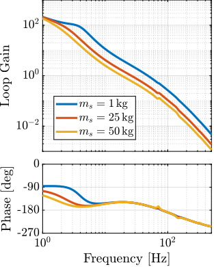
Figure 32: Loop Gain - High Authority Controller for all three nano-hexapod stiffnesses (soft one in blue, moderately stiff in red and very stiff in yellow) and all sample masses (corresponding to the three curves of each color)
6.3. Closed-Loop Noise Budgeting
The high authority position feedback controllers are then implemented and the closed-loop sensitivity to disturbances are computed. These are compared with the open-loop and damped plants cases in Figure fig:uniaxial_sensitivity_dist_hac_lac for just one configuration (moderately stiff nano-hexapod with 25kg sample’s mass). As expected, the sensitivity to disturbances is decreased in the controller bandwidth and slightly increase outside this bandwidth.

Figure 33: Change of sensitivity to disturbances with LAC and with HAC-LAC
The cumulative amplitude spectrum of the motion \(d\) is computed for all nano-hexapod configurations, all sample masses and in the open-loop (OL), damped (IFF) and position controlled (HAC-IFF) cases. The results are shown in Figure fig:uniaxial_cas_hac_lac. Obtained root mean square values of the distance \(d\) are better for the soft nano-hexapod (\(\approx 25\,nm\) to \(\approx 35\,nm\) depending on the sample’s mass) than for the stiffer nano-hexapod (from \(\approx 30\,nm\) to \(\approx 70\,nm\)).

Figure 34: Cumulative Amplitude Spectrum for all three nano-hexapod stiffnesses - Comparison of OL, IFF and HAC-LAC cases
7. Conclusion
In this study, a uniaxial model of the nano-active-stabilization-system has been tuned both from dynamical measurements (Section sec:micro_station_model) and from disturbances measurements (Section sec:uniaxial_disturbances).
It has been shown that three active damping techniques can be used to critically damp the nano-hexapod resonances (Section sec:uniaxial_active_damping). However, this model does not allows to determine which one is most suited to this application.
Finally, position feedback controllers have been developed for three considered nano-hexapod stiffnesses. These controllers were shown to be robust to the change of sample’s masses, and to provide good rejection of disturbances. It has been found that having a soft nano-hexapod makes the plant dynamics easier to control (because decoupled from the micro-station dynamics) and requires less position feedback bandwidth to fulfill the requirements. The moderately stiff nano-hexapod (\(k_n = 1\,N/\mu m\)) is requiring a bit more position feedback bandwidth, but it still seems to give acceptable results. However, the stiff nano-hexapod is the most complex to control and gives the worst positioning performances.