Unidirectional Model - Report
Table of Contents
This report is also available as a pdf.
(let ((org-export-before-parsing-hook (lambda (backend)
                                        (let* ((data (org-element-parse-buffer))
                                               (headline-labels (append
                                                                 (org-element-map data 'headline
                                                                   (lambda (hl)
                                                                     (when (org-element-property :CUSTOM_ID hl)
                                                                       (org-element-property :CUSTOM_ID hl))))
                                                                 (org-element-map data 'link
                                                                   (lambda (lnk)
                                                                     (when
                                                                         (and (string= "label" (org-element-property :type lnk))
                                                                              (eq 'headline (car (org-element-property :parent lnk))))
                                                                       (org-element-property :path lnk))))))
                                               (table-labels (append
                                                              (org-element-map data 'table
                                                                (lambda (tbl)
                                                                  (when (org-element-property :name tbl)
                                                                    (org-element-property :name tbl))))
                                                              (org-element-map data 'link
                                                                (lambda (lnk)
                                                                  (when (and (string= "label" (org-element-property :type lnk))
                                                                             (eq 'table (car (org-element-property :parent lnk))))
                                                                    (org-element-property :path lnk)))))))
                                          ;; now we need to map over these and replace them
                                          (mapc (lambda (label)
                                                  (goto-char (point-min))
                                                  (while (re-search-forward (format "ref:%s" label) nil t)
                                                    (replace-match (format "[[%s]]" label))))
                                                headline-labels)
                                          (mapc (lambda (label)
                                                  (goto-char (point-min))
                                                  (while (re-search-forward (format "label:%s" label) nil t)
                                                    (replace-match (format "<<%s>>" label))))
                                                headline-labels)
                                          (mapc (lambda (label)
                                                  (goto-char (point-min))
                                                  (while (re-search-forward (format "ref:%s" label) nil t)
                                                    (replace-match (format "[[%s]]" label))))
                                                table-labels)))))

  (org-open-file (org-html-export-to-html)))
The report is organized as follow:
- section sec:micro_station_model: an uniaxial of the micro-station is developped and compared with measurements.
- section sec:nano_station_model: a model of the NASS is added on top of the model of the micro-station and some properties of the obtained model are studied.
- section sec:noise_budget: after a definition of the control objective, an open loop noise budgeting is done. It consists of studying the effect of the sources of perturbation on the control objective. Some conclusions can be made on the open loop performances of both systems.
- section sec:active_damping: active damping is applied on the system using integral force feedback in order to obtain critical damping of the NASS’s mode.
- section sec:feedback_control: feedback control is applied using both actuators.
1. Micro Station Model
In this section, a uni-axial model of the micro-station is tuned in order to match measurements made on the micro-station
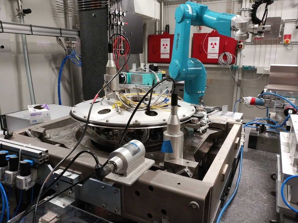
Figure 1: Experimental Setup for the first dynamical measurements on the Micro-Station. Geophones are fixed to the micro-station, and the granite as well as the micro-hexapod’s top platform are impact with an instrumented hammer
1.1. Measured dynamics
The measurement setup is schematically shown in Figure 2 where:
- Two hammer hits are performed, one on the Granite, and one on the micro-hexapod’s top platform
- The inertial motion of the granite and the micro-hexapod’s top platform are measured using geophones.
From the forces applied by the instrumented hammer and the responses of the geophones, the following frequency response functions can be computed:
- from \(F_h\) to \(d_h\) (i.e. the compliance of the micro-station)
- from \(F_g\) to \(d_h\) (or from \(F_h\) to \(d_g\))
- from \(F_g\) to \(d_g\)
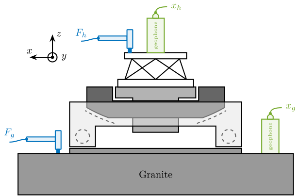
Figure 2: Measurement setup - Schematic
Due to the bad coherence at low frequency, the frequency response functions are only shown between 20 and 200Hz (Figure 3).
%% Load measured FRF
load('meas_microstation_frf.mat');

Figure 3: Measured Frequency Response Functions in the vertical direction
1.2. Uniaxial Model
The uni-axial model of the micro-station is shown in Figure 5, with:
- Disturbances:
- \(x_f\): Floor motion
- \(f_t\): Stage vibrations
- Hammer impacts: \(F_h\) and \(F_g\).
- Geophones: \(x_h\) and \(x_g\)

Figure 4: Uni-axial model of the micro-station
Masses are estimated from the CAD.
%% Parameters - Mass
mh = 15;   % Micro Hexapod [kg]
mt = 1200; % Ty + Ry + Rz [kg]
mg = 2500; % Granite [kg]
And stiffnesses from the data-sheet of stage manufacturers.
%% Parameters - Stiffnesses
kh = 6.11e+07; % [N/m]
kt = 5.19e+08; % [N/m]
kg = 9.50e+08; % [N/m]
1.3. Comparison of the model and measurements
The comparison between the measurements and the model is done in Figure 5.
Ad the model is simplistic, the goal is not to match exactly the measurement but to have a first approximation. More accurate models will be developed and tuned later on.

Figure 5: Comparison of the measured FRF and identified ones from the uni-axial model
2. Nano-Hexapod Model
A model of the nano-hexapod and sample is now added on top of the uni-axial model of the micro-station (Figure 6).
Disturbances (shown in red) are:
- \(f_s\): direct forces applied to the sample (for instance cable forces)
- \(f_t\): disturbances coming from the imperfect stage scanning performances
- \(x_f\): floor motion
The control signal is the force applied by the nano-hexapod \(f\) and the measurement is the relative motion between the sample and the granite \(d\).

Figure 6: Uni-axial model of the micro-station with added nano-hexapod and sample
2.1. Nano-Hexapod Parameters
The parameters for the nano-hexapod and sample are:
- \(m_s\) the sample mass that can vary from 1kg up to 50kg
- \(m_n\) the nano-hexapod mass which is set to 15kg
- \(k_n\) the nano-hexapod stiffness, which can vary depending on the chosen architecture/technology
As a first example, let’s choose a nano-hexapod stiffness of \(10\,N/\mu m\) and a sample mass of 10kg.
%% Nano-Hexapod Parameters
mn = 15; % [kg]
kn = 1e7; % [N/m]
cn = 2*0.01*sqrt(mn*kn); % [N/(m/s)]

%% Sample Mass
ms = 10; % [kg]
2.2. Obtained Dynamics
The sensitivity to disturbances (i.e. \(x_f\), \(f_t\) and \(f_s\)) are shown in Figure 7. The plant (i.e. the transfer function from actuator force \(f\) to measured displacement \(d\)) is shown in Figure 8.
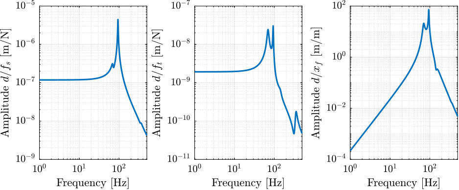
Figure 7: Sensitivity to disturbances
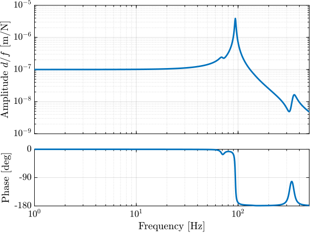
Figure 8: Bode Plot of the transfer function from actuator forces to measured displacement by the metrology
3. Disturbance Identification
In order to measure disturbances, two geophones are used, on located on the floor and on on the micro-hexapod’s top platform (see Figure 9).
The geophone on the floor is used to measured the floor motion \(x_f\) while the geophone on the micro-hexapod is used to measure vibrations introduced by scanning of the \(T_y\) stage and \(R_z\) stage.
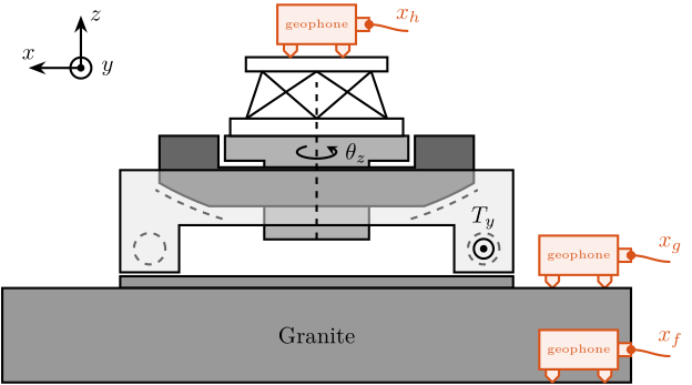
Figure 9: Disturbance measurement setup - Schematic
The voltage generated by each geophone is amplified using a voltage amplifier (gain of 60dB) before going to the ADC.
3.1. Ground Motion
The geophone fixed to the floor to measure the floor motion.
%% Load floor motion data
load('ground_motion_measurement.mat', 't', 'V');
The sensitivity of the geophone as well as the gain of the voltage amplifier are taken into account to reconstruct the floor displacement.
%% Sensitivity of the geophone
S0 = 88; % Sensitivity [V/(m/s)]
f0 = 2; % Cut-off frequency [Hz]

S = S0*(s/2/pi/f0)/(1+s/2/pi/f0); % Geophone's transfer function [V/(m/s)]

%% Gain of the voltage amplifier
G0_db = 60; % [dB]
G0 = 10^(G0_db/20); % [abs]

%% Transfer function from measured voltage to displacement
G_geo = 1/S/G0/s; % [m/V]
The PSD \(S_{V_f}\) of the measured voltage \(V_f\) is computed.
%% Compute measured voltage PSD
Fs = 1/(t(2)-t(1)); % Sampling Frequency [Hz]
win = hanning(ceil(2*Fs)); % Hanning window

[psd_V, f] = pwelch(V, win, [], [], Fs); % [V^2/Hz]
The PSD of the corresponding displacement can be computed as follows:
\begin{equation} S_{x_f}(\omega) = \frac{S_{V_f}(\omega)}{|S_{\text{geo}}(j\omega)| \cdot G_{\text{amp}} \cdot \omega} \end{equation}with:
- \(S_{\text{geo}}\) the sensitivity of the Geophone in \([Vs/m]\)
- \(G_{\text{amp}}\) the gain of the voltage amplifier
- \(\omega\) is here to integrate and have the displacement instead of the velocity
%% Ground Motion ASD
psd_xf = psd_V.*abs(squeeze(freqresp(G_geo, f, 'Hz'))).^2; % [m^2/Hz]
The amplitude spectral density \(\Gamma_{x_f}\) of the measured displacement \(x_f\) is shown in Figure 10.
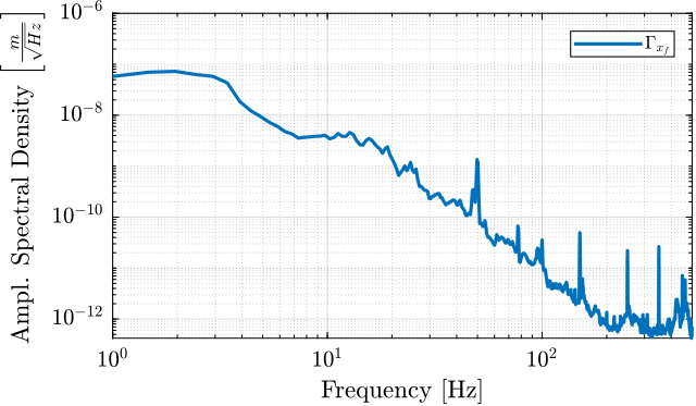
Figure 10: Measured Amplitude Spectral Density of the Floor motion on ID31
3.2. Stage Vibration
During Spindle rotation (here at 6rpm), the granite velocity and micro-hexapod’s top platform velocity are measured with the geophones.
%% Measured velocity of granite and hexapod during spindle rotation
load('meas_spindle_on.mat', 't', 'vg', 'vh');
The Power Spectral Density of the relative velocity between the hexapod and the granite is computed.
%% Compute Power Spectral Density of the relative velocity between granite and hexapod during spindle rotation
Fs = 1/(t(2)-t(1)); % Sampling Frequency [Hz]
win = hanning(ceil(2*Fs)); % Hanning window

[psd_vft, f] = pwelch(vh-vg, win, [], [], Fs); % [(m/s)^2/Hz]
It is then integrated to obtain the Amplitude Spectral Density of the relative motion (Figure 11).
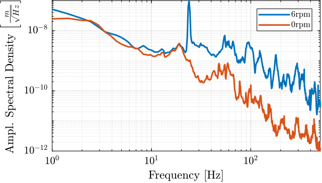
Figure 11: Measured Amplitude Spectral Density of the relative motion between the granite and the micro-hexapod’s top platform during Spindle rotating
In order to compute the equivalent disturbance force \(f_t\) that induces such motion, the transfer function from \(f_t\) to the relative motion of the hexapod’s top platform and the granite is extracted from the model. The power spectral density \(\Gamma_{f_{t}}\) of the disturbance force can be computed as follows:
\begin{equation} \Gamma_{f_{t}}(\omega) = \frac{\Gamma_{v_{t}}(\omega)}{|G_{\text{model}}(j\omega)|^2} \end{equation}with:
- \(\Gamma_{v_{t}}\) the measured power spectral density of the relative motion between the micro-hexapod’s top platform and the granite during the spindle’s rotation
- \(G_{\text{model}}\) the transfer function (extracted from the uniaxial model) from \(f_t\) to the relative motion between the micro-hexapod’s top platform and the granite
%% Power Spectral Density of the equivalent force ft
psd_ft = (psd_vft./(2*pi*f).^2)./abs(squeeze(freqresp(G('Dh', 'ft') - G('Dg', 'ft'), f, 'Hz'))).^2;
The obtained amplitude spectral density of the disturbance force \(f_t\) is shown in Figure 12.
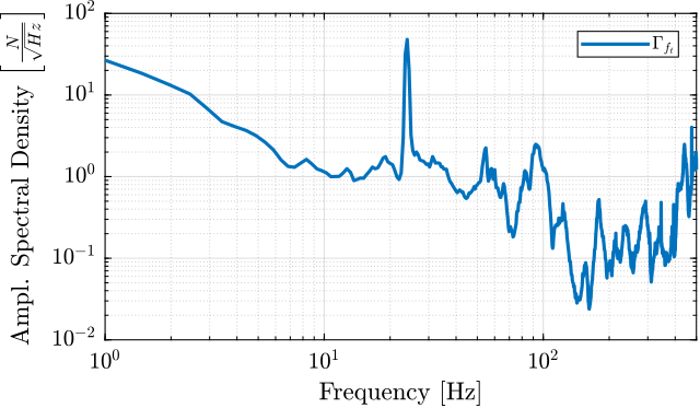
Figure 12: Estimated disturbance force ft from measurement and uniaxial model
4. Open-Loop Dynamic Noise Budgeting
Now that we have a model of the NASS and an estimation of the power spectral density of the disturbances, it is possible to perform an open-loop dynamic noise budgeting.
4.1. Sensitivity to disturbances
From the Uni-axial model, the transfer function from the disturbances (\(f_s\), \(x_f\) and \(f_t\)) to the displacement \(d\) are computed.
This is done for two extreme sample masses \(m_s = 1\,\text{kg}\) and \(m_s = 50\,\text{kg}\) and three nano-hexapod stiffnesses:
- \(k_n = 0.01\,N/\mu m\) that could represent a voice coil actuator with soft flexible guiding
- \(k_n = 1\,N/\mu m\) that could represent a voice coil actuator with a stiff flexible guiding or a mechanically amplified piezoelectric actuator
- \(k_n = 100\,N/\mu m\) that could represent a stiff piezoelectric stack actuator
The obtained sensitivity to disturbances for the three nano-hexapod stiffnesses are shown in Figure 13 for the light sample (same conclusions can be drawn with the heavy one).
From Figure 13, following can be concluded for the soft nano-hexapod:
- It is more sensitive to forces applied on the sample (cable forces for instance), which is expected due to the lower stiffness
- Between the suspension mode of the nano-hexapod (here at 5Hz) and the first mode of the micro-station (here at 70Hz), the disturbances induced by the stage vibrations are filtered out.
- Above the suspension mode of the nano-hexapod, the sample’s motion is unaffected by the floor motion, and therefore the sensitivity to floor motion is almost \(1\).

Figure 13: Sensitivity to disturbances for three different nano-hexpod stiffnesses
4.2. Open-Loop Dynamic Noise Budgeting
Now, the power spectral density of the disturbances is taken into account to estimate the residual motion \(d\) in each case.
The Cumulative Amplitude Spectrum of the relative motion \(d\) due to both the floor motion \(x_f\) and the stage vibrations \(f_t\) are shown in Figure 14 for the three nano-hexapod stiffnesses.
It is shown that the effect of the floor motion is much less than the stage vibrations, except for the soft nano-hexapod below 5Hz.

Figure 14: Cumulative Amplitude Spectrum of the relative motion d, due to both the floor motion and the stage vibrations (light sample)
The total cumulative amplitude spectrum for the three nano-hexapod stiffnesses and for the two sample’s masses are shown in Figure 15. The conclusion is that the sample’s mass has little effect on the cumulative amplitude spectrum of the relative motion \(d\).

Figure 15: Cumulative Amplitude Spectrum of the relative motion d due to all disturbances, for two sample masses
The conclusion is that in order to have a closed-loop residual vibration \(d \approx 20\,nm\text{ rms}\), if a simple feedback controller is used, the required closed-loop bandwidth would be:
- \(\approx 10\,\text{Hz}\) for the soft nano-hexapod (\(k_n = 0.01\,N/\mu m\))
- \(\approx 50\,\text{Hz}\) for the relatively stiff nano-hexapod (\(k_n = 1\,N/\mu m\))
- \(\approx 100\,\text{Hz}\) for the stiff nano-hexapod (\(k_n = 100\,N/\mu m\))
5. Active Damping
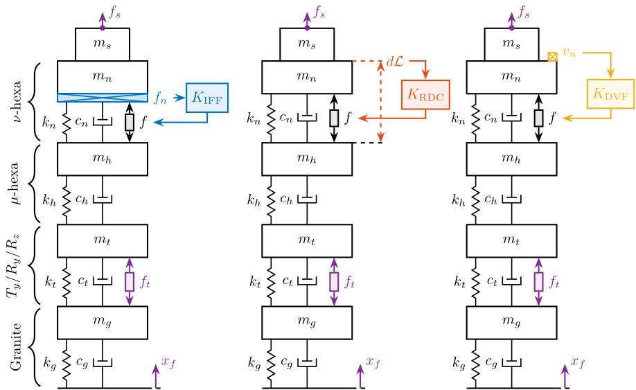
Figure 16: Three active damping strategies: Direct Velocity Feedback (DVF) using a geophone, Integral Force Feedback (IFF) using a force sensor, and Relative Motion Control (RMC) using a relative displacement sensor
5.1. Plant Dynamics
The plant dynamics for all three active damping techniques are shown in Figure 17.
All have alternating poles and zeros.
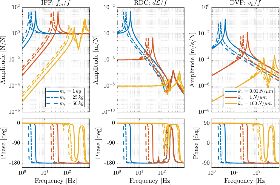
Figure 17: Plant dynamics for the three active damping techniques
5.2. Achievable Damping
Controller used for the three active damping techniques are:
\begin{align} K_{\text{IFF}}(s) &= \frac{g_{\text{IFF}}}{s} \\ K_{\text{RMC}}(s) &= g_{\text{RMC}} s \\ K_{\text{DVF}}(s) &= g_{\text{DVF}} \end{align}It is shown in the Root Locus in Figure 18 that all three active damping approach can lead to critical damping.
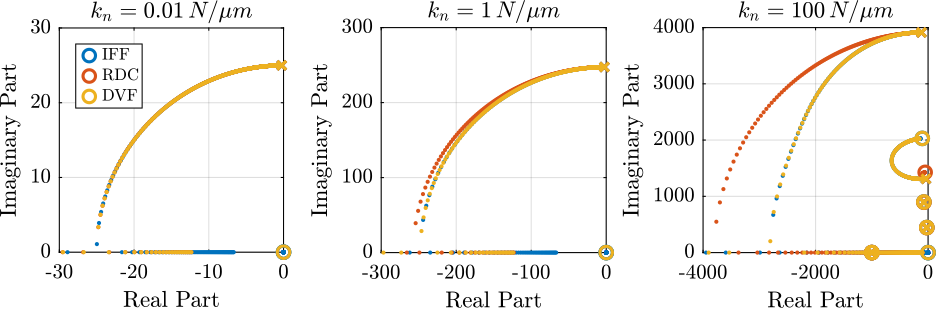
Figure 18: Root Locus for the three damping techniques
5.3. Change of sensitivity to disturbances
The sensitivity to disturbances (\(f_s\), \(f_t\) and \(x_f\)) for all three active damping techniques are compared in Figure 19.
Conclusions from Figure 19 are:
- IFF degrades the sensitivity to direct forces on the sample (i.e. the compliance) below the resonance of the nano-hexapod
- RMC degrades the sensitivity to stage vibrations around the nano-hexapod’s resonance as compared to the other two methods
- both IFF and DVF degrades the sensitivity to floor motion below the resonance of the nano-hexapod
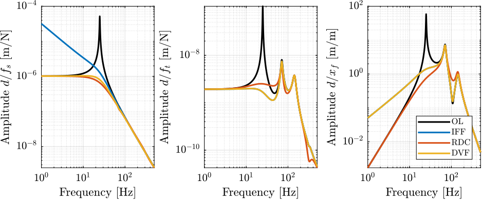
Figure 19: Change of sensitivity to disturbance with all three active damping strategies
5.4. Noise Budgeting after Active Damping
Cumulative Amplitude Spectrum of the distance \(d\) with all three active damping techniques are compared in Figure 20. All three active damping methods are giving similar results.
Active Damping helps to lower the vibrations and less bandwidth is required for the position controller.
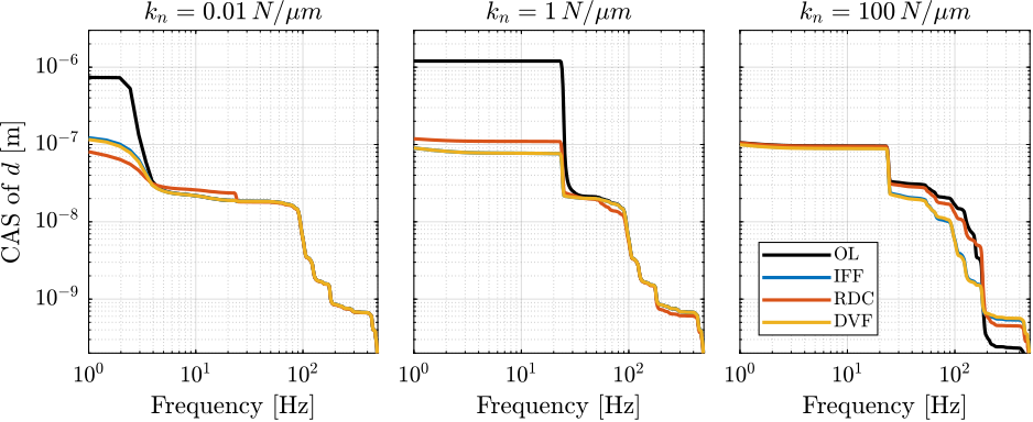
Figure 20: Cumulative Amplitude Spectrum of the distance \(d\) with all three active damping techniques
6. Position Feedback Controller
[X]Explain the HAC-LAC control strategy[ ]Show the plant for the three stiffnesses[ ]Estimate the required bandwidth to attain the specifications
The High Authority Control - Low Authority Control (HAC-LAC) architecture is shown in Figure 21. It corresponds to a two step control strategy:
- First, an active damping controller \(\bm{K}_{\textsc{LAC}}\) is implemented (see Section sec:uniaxial_active_damping). It allows to reduce the vibration level, and it also makes the damped plant (transfer function from \(u^{\prime}\) to \(y\)) easier to control than the undamped plant (transfer function from \(u\) to \(y\)).
- Then, a position controller \(K_{\textsc{HAC}}\) is implemented.
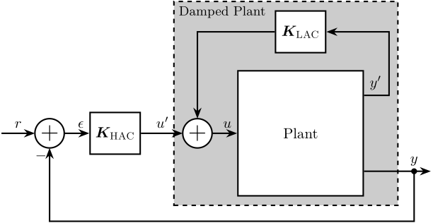
Figure 21: High Authority Control - Low Authority Control (HAC-LAC) architecture