phd-micro-station-modal-analysis/modal-analysis.org

Micro-Station - Modal Analysis

• Glossary and Acronyms - Tables
• Introduction
• Measurement Setup
  • Introduction
  • Used Instrumentation
  • Structure Preparation and Test Planing
  • Location of the Accelerometers
  • Hammer Impacts
  • Force and Response signals
• Frequency Analysis
  • Introduction
  • From accelerometer DOFs to solid body DOFs
  • Verification of solid body assumption
• Modal Analysis
  • Introduction
  • Number of modes determination
  • Modal parameter extraction
  • Verification of the modal model validity
• Conclusion
• Bibliography
• Glossary
• Footnotes

Glossary and Acronyms - Tables   ignore

label	name	description
psdx	\ensuremath{Φx}	Power spectral density of signal $x$
asdx	\ensuremath{Γx}	Amplitude spectral density of signal $x$
cpsx	\ensuremath{Φx}	Cumulative Power Spectrum of signal $x$
casx	\ensuremath{Γx}	Cumulative Amplitude Spectrum of signal $x$

key	abbreviation	full form
nass	NASS	Nano Active Stabilization System
asd	ASD	Amplitude Spectral Density
psd	PSD	Power Spectral Density
frf	FRF	Frequency Response Function
dof	DoF	Degree of freedom
svd	SVD	Singular Value Decomposition
mif	MIF	Mode Indicator Functions

Introduction   ignore

To further improve the accuracy of the performance predictions, a model that better represents the micro-station dynamics is required. A multi-body model consisting of several rigid bodies connected by kinematic constraints (i.e. joints), springs and damper elements is a good candidate to model the micro-station.

Although the inertia of each solid body can easily be estimated from its geometry and material density, it is more difficult to properly estimate the stiffness and damping properties of the guiding elements connecting each solid body. Experimental modal analysis will be used to tune the model, and to verify that a multi-body model can accurately represent the dynamics of the micro-station.

The tuning approach for the multi-body model based on measurements is illustrated in Figure ref:fig:modal_vibration_analysis_procedure. First, a response model is obtained, which corresponds to a set of frequency response functions computed from experimental measurements. From this response model, the modal model can be computed, which consists of two matrices: one containing the natural frequencies and damping factors of the considered modes, and another describing the mode shapes. This modal model can then be used to tune the spatial model (i.e. the multi-body model), that is, to tune the mass of the considering solid bodies and the springs and dampers connecting the solid bodies.

\begin{tikzpicture}
  \node[block, inner sep = 8pt, align=center] (1) {Description\\of structure};
  \node[block, inner sep = 8pt, align=center, left=1.0 of 1] (2) {Vibration\\Modes};
  \node[block, inner sep = 8pt, align=center, left=1.0 of 2] (3) {Response\\Levels};

  \draw[<->] (1) -- (2);
  \draw[<->] (2) -- (3);

  \node[above] (labelt) at (1.north) {Spatial Model};
  \node[] at (2|-labelt) {Modal Model};
  \node[] at (3|-labelt) {Response Model};

  \node[align = center, font=\tiny, below] (labelb) at (1.south) {Mass\\Stiffness\\Damping};
  \node[align = center, font=\tiny] at (2|-labelb) {Natural Frequencies\\Mode Shapes\\};
  \node[align = center, font=\tiny] at (3|-labelb) {Time Responses\\Frequency Responses\\};
\end{tikzpicture}

Three models of the same structure. The goal is to tune a spatial model (i.e. mass, stiffness and damping properties) from a response model. The modal model can be used as an intermediate step.

The measurement setup used to obtain the response model is described in Section ref:sec:modal_meas_setup. This includes the instrumentation used (i.e. instrumented hammer, accelerometers and acquisition system), test planing, and a first analysis of the obtained signals.

In Section ref:sec:modal_frf_processing, the obtained frequency response functions between the forces applied by the instrumented hammer and the accelerometers fixed to the structure are computed. These measurements are projected at the center of mass of each considered solid body to facilitate the further use of the results. The solid body assumption is then verified, validating the use of the multi-body model.

Finally, the modal analysis is performed in Section ref:sec:modal_analysis. This shows how complex the micro-station dynamics is, and the necessity of having a model representing its complex dynamics.

Measurement Setup

<<sec:modal_meas_setup>>

Introduction   ignore

In order to perform an experimental modal analysis, a suitable measurement setup is essential. This includes using appropriate instrumentation (presented in Section ref:ssec:modal_instrumentation) and properly preparing the structure to be measured (Section ref:ssec:modal_test_preparation). Then, the locations of the measured motions (Section ref:ssec:modal_accelerometers) and the locations of the hammer impacts (Section ref:ssec:modal_hammer_impacts) have to be chosen carefully. The obtained force and acceleration signals are described in Section ref:ssec:modal_measured_signals, and the quality of the measured data is assessed.

Used Instrumentation

<<ssec:modal_instrumentation>>

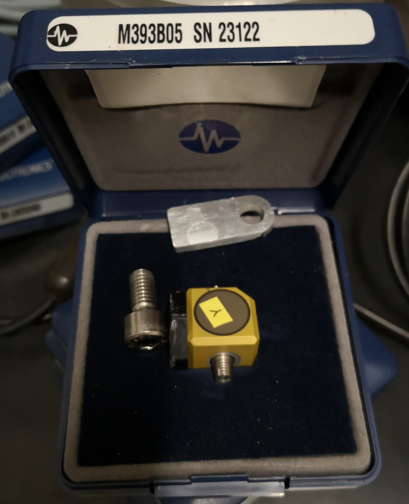
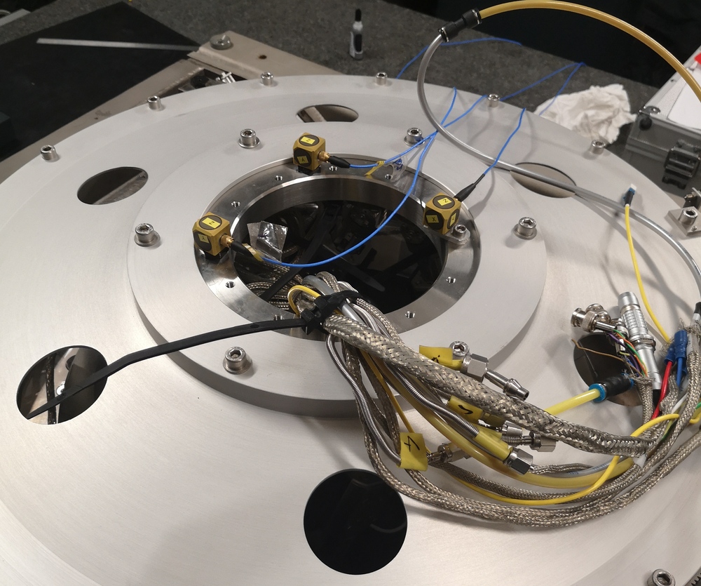
Three type of equipment are essential for a good modal analysis. First, accelerometers are used to measure the response of the structure. Here, 3-axis accelerometers¹ shown in figure ref:fig:modal_accelero_M393B05 are used. These accelerometers were glued to the micro-station using a thin layer of wax for best results cite:&ewins00_modal chapt. 3.5.7.

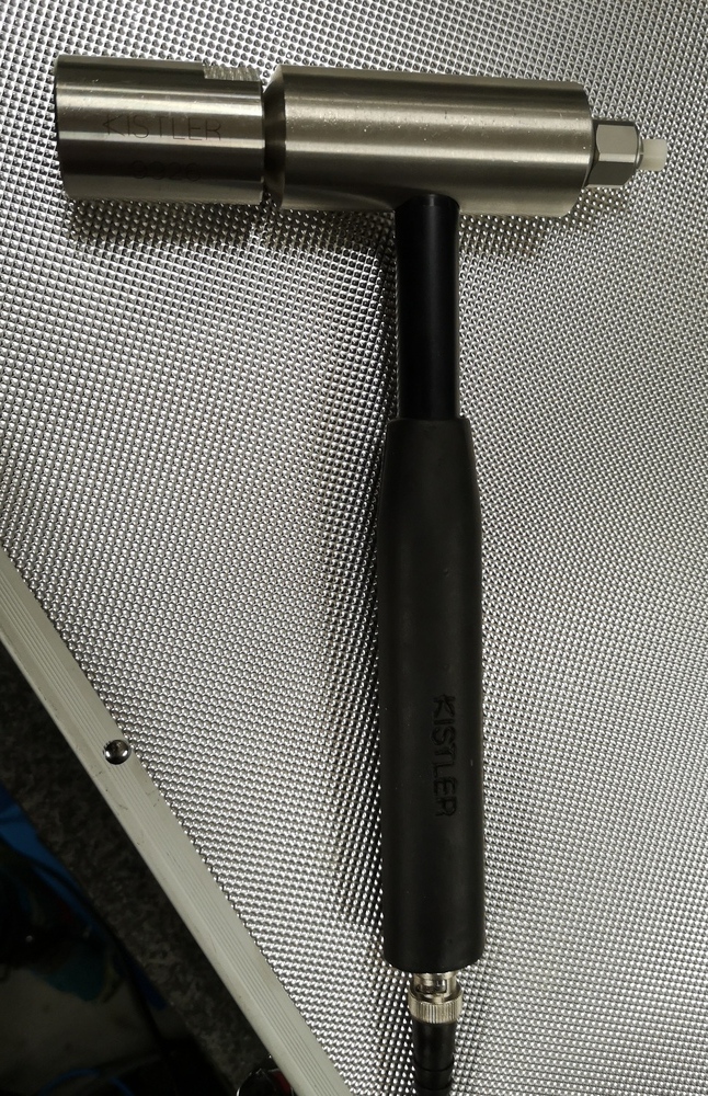
Then, an instrumented hammer² (figure ref:fig:modal_instrumented_hammer) is used to apply forces to the structure in a controlled manner. Tests were conducted to determine the most suitable hammer tip (ranging from a metallic one to a soft plastic one). The softer tip was found to give best results as it injects more energy in the low-frequency range where the coherence was low, such that the overall coherence was improved.

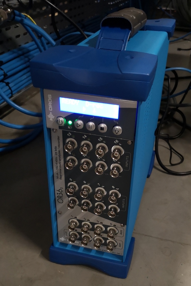
Finally, an acquisition system³ (figure ref:fig:modal_oros) is used to acquire the injected force and response accelerations in a synchronized manner and with sufficiently low noise.

Structure Preparation and Test Planing

<<ssec:modal_test_preparation>>

To obtain meaningful results, the modal analysis of the micro-station in performed in-situ. To do so, all the micro-station stage controllers are turned "ON". This is especially important for stages for which the stiffness is provided by local feedback control, such as the air bearing spindle, and the translation stage. If these local feedback controls were turned OFF, this would have resulted in very low-frequency modes that were difficult to measure in practice, and it would also have led to decoupled dynamics, which would not be the case in practice.

The top part representing the active stabilization stage was disassembled as the active stabilization stage will be added in the multi-body model afterwards.

To perform the modal analysis from the measured responses, the $n \times n$ frequency response function matrix $\mathbf{H}$ needs to be measured, where $n$ is the considered number of degrees of freedom. The $H_{jk}$ element of this acrfull:frf matrix corresponds to the frequency response function from a force $F_k$ applied at acrfull:dof $k$ to the displacement of the structure $X_j$ at acrshort:dof $j$. Measuring this acrshort:frf matrix is time consuming as it requires to make $n \times n$ measurements. However, due to the principle of reciprocity ($H_{jk} = H_{kj}$) and using the point measurement ($H_{jj}$), it is possible to reconstruct the full matrix by measuring only one column or one line of the matrix $\mathbf{H}$ cite:&ewins00_modal chapt. 5.2. Therefore, a minimum set of $n$ frequency response functions is required. This can be done either by measuring the response $X_{j}$ at a fixed acrshort:dof $j$ while applying forces $F_{i}$ for at all $n$ considered acrshort:dof, or by applying a force $F_{k}$ at a fixed acrshort:dof $k$ and measuring the response $X_{i}$ for all $n$ acrshort:dof.

It is however not advised to measure only one row or one column, as one or more modes may be missed by an unfortunate choice of force or acceleration measurement location (for instance if the force is applied at a vibration node of a particular mode). In this modal analysis, it is chosen to measure the response of the structure at all considered acrshort:dof, and to excite the structure at one location in three directions in order to have some redundancy, and to ensure that all modes are properly identified.

Location of the Accelerometers

<<ssec:modal_accelerometers>>

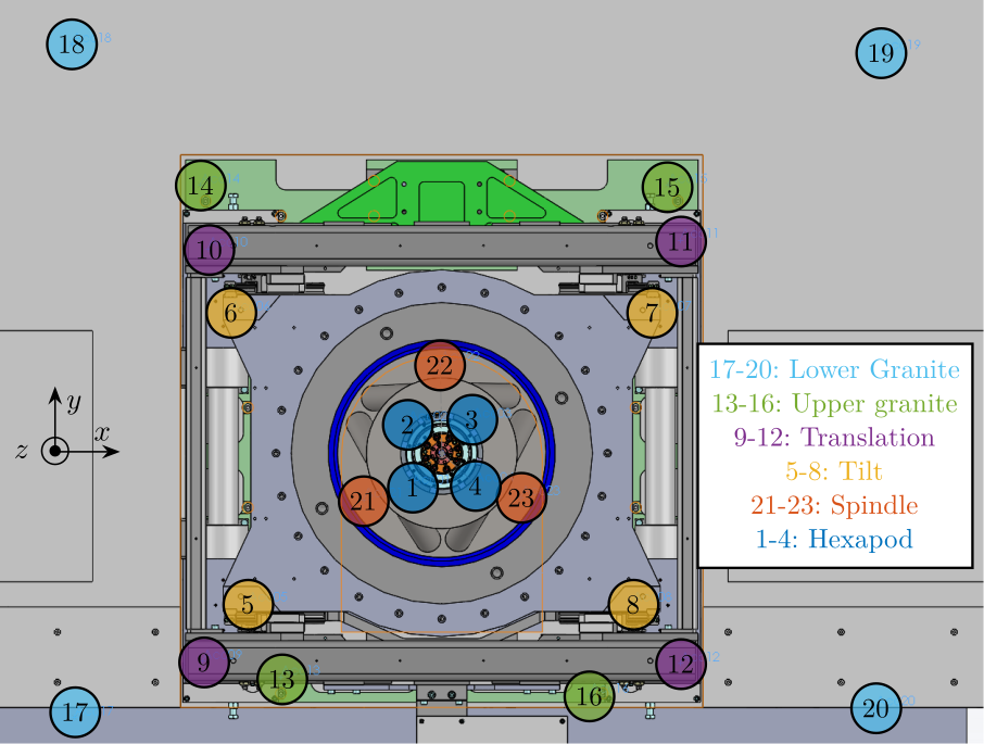
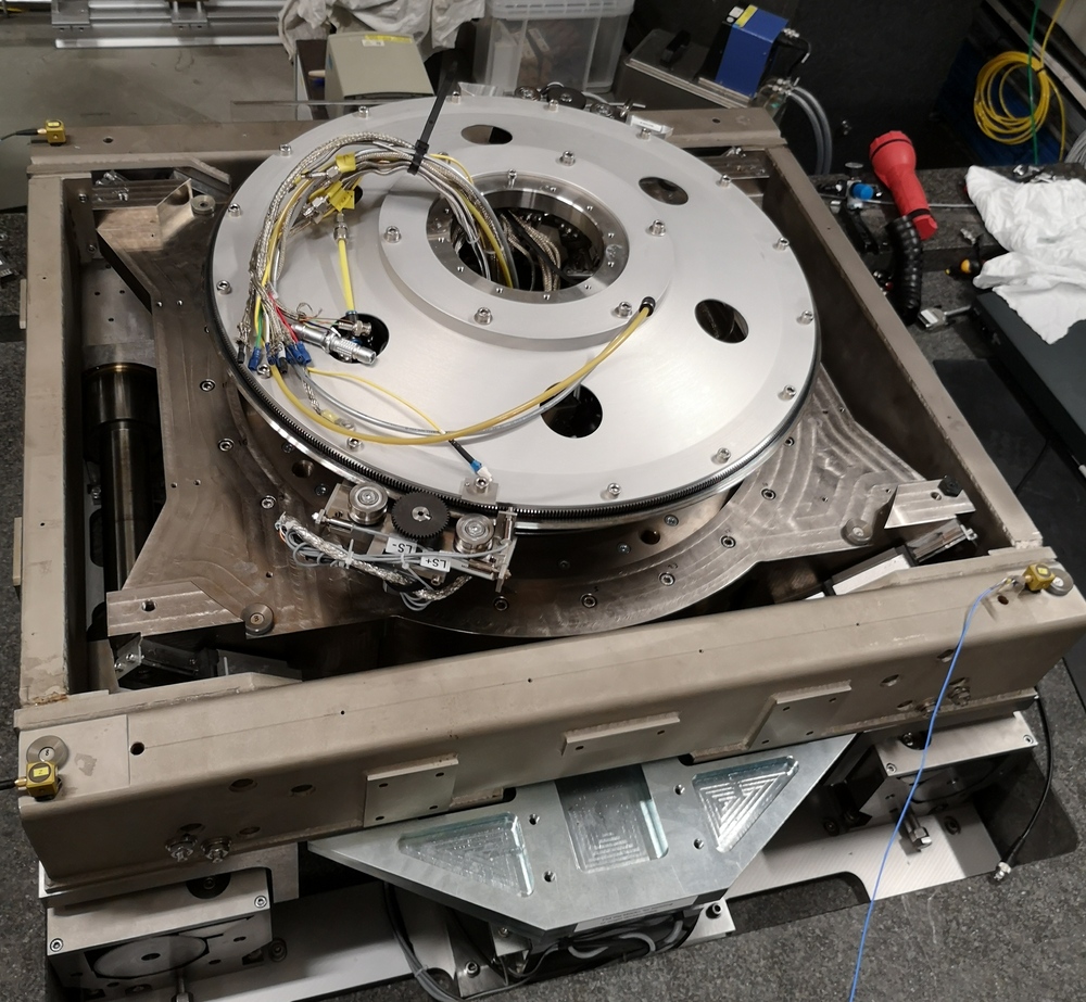
The location of the accelerometers fixed to the micro-station is essential because it defines where the dynamics is measured. A total of 23 accelerometers were fixed to the six key stages of the micro station: the lower and upper granites, the translation stage, the tilt stage, the spindle and the micro hexapod. The positions of the accelerometers are visually shown on a CAD model in Figure ref:fig:modal_location_accelerometers and their precise locations with respect to a frame located at the point of interest are summarized in Table ref:tab:modal_position_accelerometers. Pictures of the accelerometers fixed to the translation stage and to the micro-hexapod are shown in Figure ref:fig:modal_accelerometer_pictures.

As all key stages of the micro-station are expected to behave as solid bodies, only 6 acrshort:dof can be considered for each solid body. However, it was chosen to use four 3-axis accelerometers (i.e. 12 measured acrshort:dof) for each considered solid body to have some redundancy and to be able to verify the solid body assumption (see Section ref:ssec:modal_solid_body_assumption).

\hfill

	$x$	$y$	$z$
(17) Low. Granite	-730	-526	-951
(18) Low. Granite	-735	814	-951
(19) Low. Granite	875	799	-951
(20) Low. Granite	865	-506	-951
(13) Up. Granite	-320	-446	-786
(14) Up. Granite	-480	534	-786
(15) Up. Granite	450	534	-786
(16) Up. Granite	295	-481	-786
(9) Translation	-475	-414	-427
(10) Translation	-465	407	-427
(11) Translation	475	424	-427
(12) Translation	475	-419	-427
(5) Tilt	-385	-300	-417
(6) Tilt	-420	280	-417
(7) Tilt	420	280	-417
(8) Tilt	380	-300	-417
(21) Spindle	-155	-90	-594
(22) Spindle	0	180	-594
(23) Spindle	155	-90	-594
(1) Hexapod	-64	-64	-270
(2) Hexapod	-64	64	-270
(3) Hexapod	64	64	-270
(4) Hexapod	64	-64	-270

%% Load Accelerometer positions
acc_pos = readtable('mat/acc_pos.txt', 'ReadVariableNames', false);
acc_pos = table2array(acc_pos(:, 1:4));
[~, i] = sort(acc_pos(:, 1));
acc_pos = acc_pos(i, 2:4);

Hammer Impacts

<<ssec:modal_hammer_impacts>>

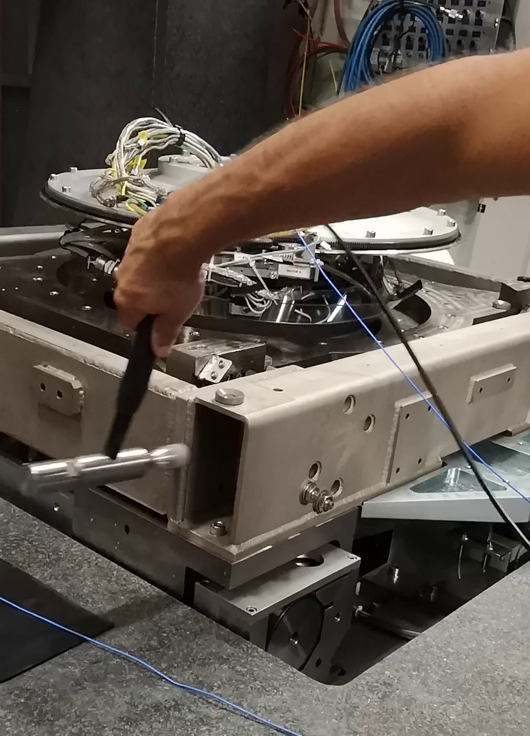
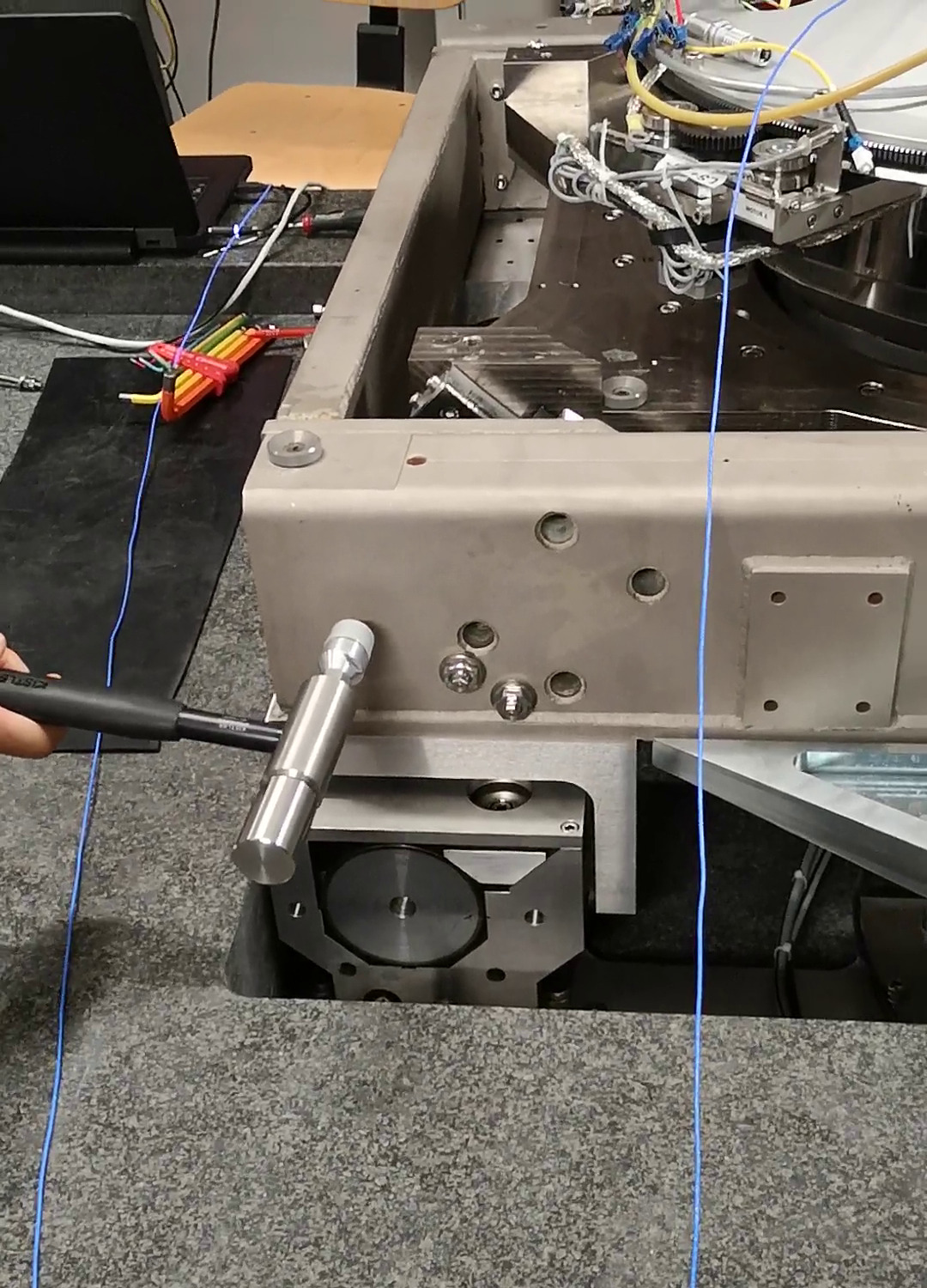
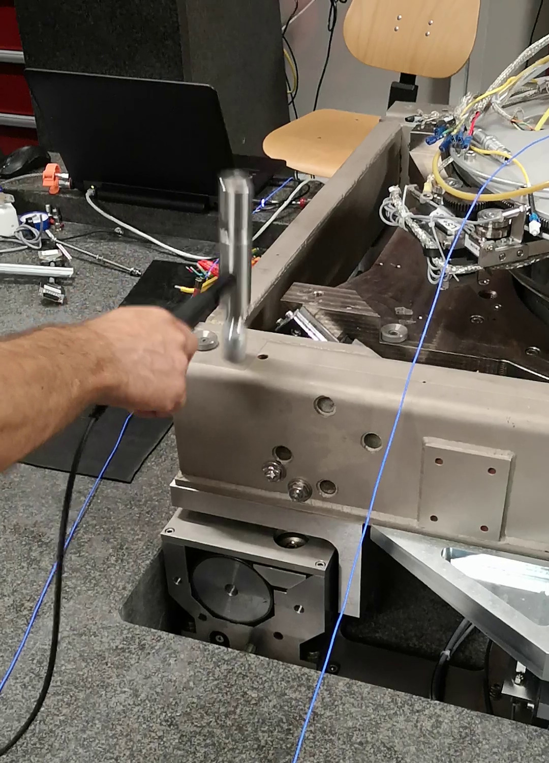
The selected location of the hammer impact corresponds to the location of accelerometer number $11$ fixed to the translation stage. It was chosen to match the location of one accelerometer, because a point measurement (i.e. a measurement of $H_{kk}$) is necessary to be able to reconstruct the full acrshort:frf matrix cite:ewins00_modal.

The impacts were performed in three directions, as shown in figures ref:fig:modal_impact_x, ref:fig:modal_impact_y and ref:fig:modal_impact_z.

Force and Response signals

<<ssec:modal_measured_signals>>

The force sensor of the instrumented hammer and the accelerometer signals are shown in the time domain in Figure ref:fig:modal_raw_meas. Sharp "impacts" can be observed for the force sensor, indicating wide frequency band excitation. For the accelerometer, a much more complex signal can be observed, indicating complex dynamics.

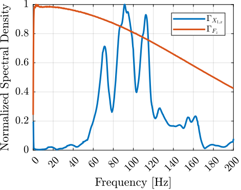
The "normalized" acrfull:asd of the two signals were computed and shown in Figure ref:fig:modal_asd_acc_force. Conclusions based on the time domain signals can be clearly observed in the frequency domain (wide frequency content for the force signal and complex dynamics for the accelerometer). These data are corresponding to an hammer impact in the vertical direction and to the measured acceleration in the $x$ direction by accelerometer $1$ (fixed to the micro-hexapod). Similar results were obtained for all measured frequency response functions.

%% Load raw data
meas1_raw = load('mat/meas_raw_1.mat');

% Sampling Frequency [Hz]
Fs = 1/meas1_raw.Track1_X_Resolution;

% Time just before the impact occurs [s]
impacts = [5.937, 11.228, 16.681, 22.205, 27.350, 32.714, 38.115, 43.888, 50.407]-0.01;

% Time vector [s]
time = linspace(0, meas1_raw.Track1_X_Resolution*length(meas1_raw.Track1), length(meas1_raw.Track1));

%% Frequency Analysis
Nfft = floor(5.0*Fs); % Number of frequency points
win = hanning(Nfft); % Windowing
Noverlap = floor(Nfft/2); % Overlap for frequency analysis

%% Comnpute the power spectral density of the force and acceleration
[pxx_force, f] = pwelch(meas1_raw.Track1, win, Noverlap, Nfft, Fs);
[pxx_acc,   ~] = pwelch(meas1_raw.Track2, win, Noverlap, Nfft, Fs);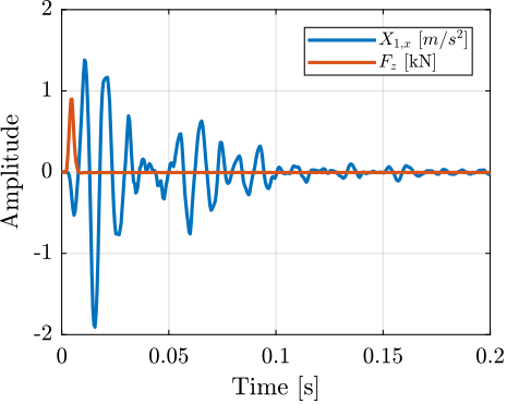

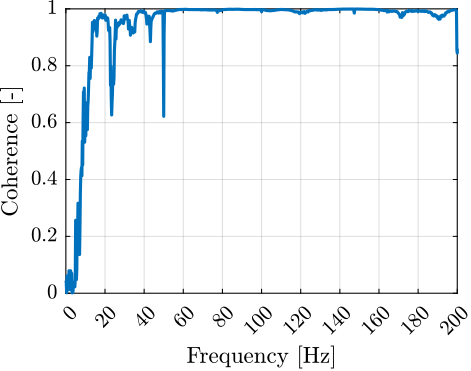
The frequency response function from the applied force to the measured acceleration is then computed and shown Figure ref:fig:modal_frf_acc_force. The quality of the obtained data can be estimated using the coherence function (Figure ref:fig:modal_coh_acc_force). Good coherence is obtained from $20\,\text{Hz}$ to $200\,\text{Hz}$ which corresponds to the frequency range of interest.

%% Compute the transfer function and Coherence
[G1,   f] = tfestimate(meas1_raw.Track1, meas1_raw.Track2, win, Noverlap, Nfft, Fs);
[coh1, ~] = mscohere(  meas1_raw.Track1, meas1_raw.Track2, win, Noverlap, Nfft, Fs);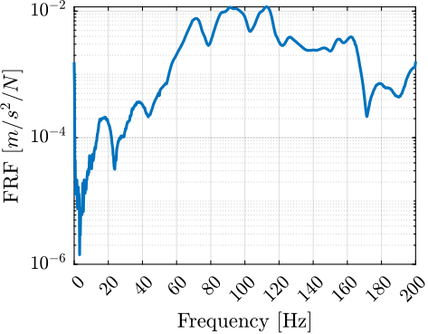

Frequency Analysis

<<sec:modal_frf_processing>>

Introduction   ignore

After all measurements are conducted, a $n \times p \times q$ acrlongpl:frf matrix can be computed with:

• $n = 69$: number of output measured acceleration (23 3-axis accelerometers)
• $p = 3$: number of input force excitation
• $q = 801$: number of frequency points $\omega_{i}$

For each frequency point $\omega_{i}$, a 2D complex matrix is obtained that links the 3 force inputs to the 69 output accelerations eqref:eq:modal_frf_matrix_raw.

\begin{equation}\label{eq:modal_frf_matrix_raw} \mathbf{H}(ω_i) = \begin{bmatrix} \frac{D_{1_x}}{F_x}(ω_i) & \frac{D_{1_x}}{F_y}(ω_i) & \frac{D_{1_x}}{F_z}(ω_i)
\frac{D_{1_y}}{F_x}(ω_i) & \frac{D_{1_y}}{F_y}(ω_i) & \frac{D_{1_y}}{F_z}(ω_i)
\frac{D_{1_z}}{F_x}(ω_i) & \frac{D_{1_z}}{F_y}(ω_i) & \frac{D_{1_z}}{F_z}(ω_i)
\frac{D_{2_x}}{F_x}(ω_i) & \frac{D_{2_x}}{F_y}(ω_i) & \frac{D_{2_x}}{F_z}(ω_i)
\vdots & \vdots & \vdots
\frac{D_{23_z}}{F_x}(ω_i) & \frac{D_{23_z}}{F_y}(ω_i) & \frac{D_{23_z}}{F_z}(ω_i) \\

\end{bmatrix}

\end{equation}

However, for the multi-body model being developed, only 6 solid bodies are considered, namely: the bottom granite, the top granite, the translation stage, the tilt stage, the spindle and the micro-hexapod. Therefore, only $6 \times 6 = 36$ degrees of freedom are of interest. Therefore, the objective of this section is to to process the Frequency Response Matrix to reduce the number of measured acrshort:dof from 69 to 36.

The coordinate transformation from accelerometers acrshort:dof to the solid body 6 acrshortpl:dof (three translations and three rotations) is performed in Section ref:ssec:modal_acc_to_solid_dof. The $69 \times 3 \times 801$ frequency response matrix is then reduced to a $36 \times 3 \times 801$ frequency response matrix where the motion of each solid body is expressed with respect to its center of mass.

To validate this reduction of acrshort:dof and the solid body assumption, the frequency response function at the accelerometer location are "reconstructed" from the reduced frequency response matrix and are compared with the initial measurements in Section ref:ssec:modal_solid_body_assumption.

From accelerometer DOFs to solid body DOFs

<<ssec:modal_acc_to_solid_dof>>

Let us consider the schematic shown in Figure ref:fig:modal_local_to_global_coordinates where the motion of a solid body is measured at 4 distinct locations (in $x$, $y$ and $z$ directions). The goal here is to link these $4 \times 3 = 12$ measurements to the 6 acrshort:dof of the solid body expressed in the frame $\{O\}$.

  \newcommand\irregularcircle[2]{% radius, irregularity
    \pgfextra {\pgfmathsetmacro\len{(#1)+rand*(#2)}}
    +(0:\len pt)
    \foreach \a in {10,20,...,350}{
      \pgfextra {\pgfmathsetmacro\len{(#1)+rand*(#2)}}
      -- +(\a:\len pt)
    } -- cycle
  }
  \begin{tikzpicture}
    \draw[rounded corners=1mm, fill=blue!30!white] (0, 0) \irregularcircle{3cm}{1mm};

    \node[] (origin) at (0, 0) {$\bullet$};
    \begin{scope}[shift={(origin)}]
      \def\axissize{0.8cm}
      \draw[->] (0, 0) -- ++(\axissize, 0) node[above left]{$x$};
      \draw[->] (0, 0) -- ++(0, \axissize) node[below right]{$y$};
      \draw[fill, color=black] (0, 0) circle (0.05*\axissize);
      \node[draw, circle, inner sep=0pt, minimum size=0.4*\axissize, label=left:$z$] (yaxis) at (0, 0){};
      \node[below right] at (0, 0){$\{O\}$};
    \end{scope}

    \coordinate[] (p1) at (-1.5, -1.5);
    \coordinate[] (p2) at (-1.5,  1.5);
    \coordinate[] (p3) at ( 1.5,  1.5);
    \coordinate[] (p4) at ( 1.5, -1.5);

    \draw[->] (p1)node[]{$\bullet$}node[above]{$\vec{p}_1$} -- ++( 1  , 0.1)node[right]{$\delta \vec{p}_1$};
    \draw[->] (p2)node[]{$\bullet$}node[above]{$\vec{p}_2$} -- ++(-0.5,-0.4)node[below]{$\delta \vec{p}_2$};
    \draw[->] (p3)node[]{$\bullet$}node[above]{$\vec{p}_3$} -- ++(-0.8,-0.1)node[below]{$\delta \vec{p}_3$};
    \draw[->] (p4)node[]{$\bullet$}node[above]{$\vec{p}_4$} -- ++( 0.5, 0.2)node[below]{$\delta \vec{p}_4$};
  \end{tikzpicture}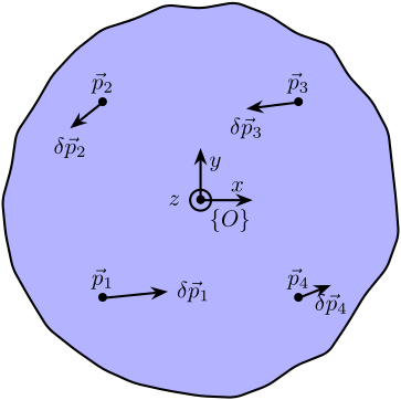

Schematic of the measured motions of a solid body

The motion of the rigid body of figure ref:fig:modal_local_to_global_coordinates can be described by its displacement $\vec{\delta}p = [\delta p_x,\ \delta p_y,\ \delta p_z]$ and (small) rotations $[\delta \Omega_x,\ \delta \Omega_y,\ \delta \Omega_z]$ with respect to the reference frame $\{O\}$.

The motion $\vec{\delta} p_{i}$ of a point $p_i$ can be computed from $\vec{\delta} p$ and $\bm{\delta \Omega}$ using equation eqref:eq:modal_compute_point_response, with $\bm{\delta\Omega}$ defined in equation eqref:eq:modal_rotation_matrix cite:&ewins00_modal chapt. 4.3.2.

\begin{equation}\label{eq:modal_compute_point_response} \vec{δ} p_i &= \vec{δ} p + \bm{δ Ω} ⋅ \vec{p}_i \\

\end{equation}

\begin{equation}\label{eq:modal_rotation_matrix} \bm{δΩ} = \begin{bmatrix} 0 & -δΩ_z & δΩ_y
δΩ_z & 0 & -δΩ_x
-δΩ_y & δΩ_x & 0

\end{bmatrix}

\end{equation}

Writing this in matrix form for the four points gives eqref:eq:modal_cart_to_acc.

\begin{equation}\label{eq:modal_cart_to_acc} ≤ft[\begin{array}{c} \delta p_{1x} \\ \delta p_{1y} \\ \delta p_{1z} \\\hline \vdots \\\hline \delta p_{4x} \\ \delta p_{4y} \\ \delta p_{4z} \end{array}\right] = \left[\begin{array}{ccc|ccc} 1 & 0 & 0 & 0 & p_{1z} & -p_{1y} \\ 0 & 1 & 0 & -p_{1z} & 0 & p_{1x} \\ 0 & 0 & 1 & p_{1y} & -p_{1x} & 0 \\ \hline & \vdots & & & \vdots & \\ \hline 1 & 0 & 0 & 0 & p_{4z} & -p_{4y} \\ 0 & 1 & 0 & -p_{4z} & 0 & p_{4x} \\ 0 & 0 & 1 & p_{4y} & -p_{4x} & 0 \end{array}\right] \left[\begin{array}{c} \delta p_x \\ \delta p_y \\ \delta p_z \\ \hline \delta\Omega_x \\ \delta\Omega_y \\ \delta\Omega_z \end{array}\right] = ≤ft[\begin{array}{ccc|ccc} 1 & 0 & 0 & 0 & p_{1z} & -p_{1y} \\ 0 & 1 & 0 & -p_{1z} & 0 & p_{1x} \\ 0 & 0 & 1 & p_{1y} & -p_{1x} & 0 \\ \hline & \vdots & & & \vdots & \\ \hline 1 & 0 & 0 & 0 & p_{4z} & -p_{4y} \\ 0 & 1 & 0 & -p_{4z} & 0 & p_{4x} \\ 0 & 0 & 1 & p_{4y} & -p_{4x} & 0 \end{array}\right] \left[\begin{array}{c} \delta p_x \\ \delta p_y \\ \delta p_z \\ \hline \delta\Omega_x \\ \delta\Omega_y \\ \delta\Omega_z \end{array}\right] ≤ft[\begin{array}{c} \delta p_x \\ \delta p_y \\ \delta p_z \\ \hline \delta\Omega_x \\ \delta\Omega_y \\ \delta\Omega_z \end{array}\right]

\end{equation}

Provided that the four sensors are properly located, the system of equation eqref:eq:modal_cart_to_acc can be solved by matrix inversion⁴. The motion of the solid body expressed in a chosen frame $\{O\}$ can be determined using equation eqref:eq:modal_determine_global_disp. Note that this matrix inversion is equivalent to resolving a mean square problem. Therefore, having more accelerometers permits better approximation of the motion of a solid body.

\begin{equation} \left[\begin{array}{c} \delta p_x \\ \delta p_y \\ \delta p_z \\ \hline \delta\Omega_x \\ \delta\Omega_y \\ \delta\Omega_z \end{array}\right] = \left[\begin{array}{ccc|ccc} 1 & 0 & 0 & 0 & p_{1z} & -p_{1y} \\ 0 & 1 & 0 & -p_{1z} & 0 & p_{1x} \\ 0 & 0 & 1 & p_{1y} & -p_{1x} & 0 \\ \hline & \vdots & & & \vdots & \\ \hline 1 & 0 & 0 & 0 & p_{4z} & -p_{4y} \\ 0 & 1 & 0 & -p_{4z} & 0 & p_{4x} \\ 0 & 0 & 1 & p_{4y} & -p_{4x} & 0 \end{array}\right]^{-1} \left[\begin{array}{c} \delta p_{1x} \\ \delta p_{1y} \\ \delta p_{1z} \\\hline \vdots \\\hline \delta p_{4x} \\ \delta p_{4y} \\ \delta p_{4z} \end{array}\right] \label{eq:modal_determine_global_disp} \end{equation}

From the CAD model, the position of the center of mass of each considered solid body is computed (see Table ref:tab:modal_com_solid_bodies). The position of each accelerometer with respect to the center of mass of the corresponding solid body can easily be determined.

%% Load frequency response matrix
load('frf_matrix.mat', 'freqs', 'frf');

%% Load Accelerometer positions
acc_pos = readtable('mat/acc_pos.txt', 'ReadVariableNames', false);
acc_pos = table2array(acc_pos(:, 1:4));
[~, i] = sort(acc_pos(:, 1));
acc_pos = acc_pos(i, 2:4);

%% Accelerometers ID connected to each solid body
solids = {};
solids.gbot = [17, 18, 19, 20]; % bottom granite
solids.gtop = [13, 14, 15, 16]; % top granite
solids.ty   = [9, 10, 11, 12]; % Ty stage
solids.ry   = [5, 6, 7, 8]; % Ry stage
solids.rz   = [21, 22, 23]; % Rz stage
solids.hexa = [1, 2, 3, 4]; % Hexapod

% Names of the solid bodies
solid_names = fields(solids);

%% Save the accelerometer positions are well as the solid bodies
save('mat/geometry.mat', 'solids', 'solid_names', 'acc_pos');

%% Save the accelerometer positions are well as the solid bodies
save('matlab/mat/geometry.mat', 'solids', 'solid_names', 'acc_pos');

%% Extract the CoM of considered solid bodies
model_com = reshape(table2array(readtable('mat/model_solidworks_com.txt', 'ReadVariableNames', false)), [3, 6]);

	$X$	$Y$	$Z$
Bottom Granite	$45\,\text{mm}$	$144\,\text{mm}$	$-1251\,\text{mm}$
Top granite	$52\,\text{mm}$	$258\,\text{mm}$	$-778\,\text{mm}$
Translation stage	$0$	$14\,\text{mm}$	$-600\,\text{mm}$
Tilt Stage	$0$	$-5\,\text{mm}$	$-628\,\text{mm}$
Spindle	$0$	$0$	$-580\,\text{mm}$
Hexapod	$-4\,\text{mm}$	$6\,\text{mm}$	$-319\,\text{mm}$

Using eqref:eq:modal_determine_global_disp, the frequency response matrix $\mathbf{H}_\text{CoM}$ eqref:eq:modal_frf_matrix_com expressing the response at the center of mass of each solid body $D_i$ ($i$ from $1$ to $6$ for the $6$ considered solid bodies) can be computed from the initial acrshort:frf matrix $\mathbf{H}$.

\begin{equation}\label{eq:modal_frf_matrix_com} \mathbf{H}_\text{CoM}(ω_i) = \begin{bmatrix} \frac{D_{1,T_x}}{F_x}(ω_i) & \frac{D_{1,T_x}}{F_y}(ω_i) & \frac{D_{1,T_x}}{F_z}(ω_i)
\frac{D_{1,T_y}}{F_x}(ω_i) & \frac{D_{1,T_y}}{F_y}(ω_i) & \frac{D_{1,T_y}}{F_z}(ω_i)
\frac{D_{1,T_z}}{F_x}(ω_i) & \frac{D_{1,T_z}}{F_y}(ω_i) & \frac{D_{1,T_z}}{F_z}(ω_i)
\frac{D_{1,R_x}}{F_x}(ω_i) & \frac{D_{1,R_x}}{F_y}(ω_i) & \frac{D_{1,R_x}}{F_z}(ω_i)
\frac{D_{1,R_y}}{F_x}(ω_i) & \frac{D_{1,R_y}}{F_y}(ω_i) & \frac{D_{1,R_y}}{F_z}(ω_i)
\frac{D_{1,R_z}}{F_x}(ω_i) & \frac{D_{1,R_z}}{F_y}(ω_i) & \frac{D_{1,R_z}}{F_z}(ω_i)
\frac{D_{2,T_x}}{F_x}(ω_i) & \frac{D_{2,T_x}}{F_y}(ω_i) & \frac{D_{2,T_x}}{F_z}(ω_i)
\vdots & \vdots & \vdots
\frac{D_{6,R_z}}{F_x}(ω_i) & \frac{D_{6,R_z}}{F_y}(ω_i) & \frac{D_{6,R_z}}{F_z}(ω_i)

\end{bmatrix}

\end{equation}

%% Frequency Response Matrix - Response expressed at the CoM of the solid bodies
frfs_CoM = zeros(length(solid_names)*6, 3, 801);

for solid_i = 1:length(solid_names)
  % Number of accelerometers fixed to this solid body
  solids_i = solids.(solid_names{solid_i});

  % "Jacobian" matrix to go from accelerometer frame to CoM frame
  A = zeros(3*length(solids_i), 6);
  for i = 1:length(solids_i)
    acc_i = solids_i(i);

    acc_pos_com = acc_pos(acc_i, :).' - model_com(:, solid_i);

    A(3*(i-1)+1:3*i, 1:3) = eye(3);
    A(3*(i-1)+1:3*i, 4:6) = [ 0               acc_pos_com(3) -acc_pos_com(2) ;
                             -acc_pos_com(3)  0               acc_pos_com(1) ;
                              acc_pos_com(2) -acc_pos_com(1)  0];
  end

  for exc_dir = 1:3
    frfs_CoM((solid_i-1)*6+1:solid_i*6, exc_dir, :) = A\squeeze(frf((solids_i(1)-1)*3+1:solids_i(end)*3, exc_dir, :));
  end
end

%% Save the computed FRF at the CoM
save('mat/frf_com.mat', 'frfs_CoM');

%% Save the computed FRF at the CoM
save('matlab/mat/frf_com.mat', 'frfs_CoM');

Verification of solid body assumption

<<ssec:modal_solid_body_assumption>>

From the response of one solid body expressed by its 6 acrshortpl:dof (i.e. from $\mathbf{H}_{\text{CoM}}$), and using equation eqref:eq:modal_cart_to_acc, it is possible to compute the response of the same solid body at any considered location. In particular, the responses at the locations of the four accelerometers can be computed and compared with the original measurements $\mathbf{H}$. This is what is done here to check whether the solid body assumption is correct in the frequency band of interest.

%% Compute the FRF at the accelerometer location from the CoM reponses
frfs_A = zeros(size(frf));

% For each excitation direction
for exc_dir = 1:3
  % For each solid
  for solid_i = 1:length(solid_names)
    v0 = squeeze(frfs_CoM((solid_i-1)*6+1:(solid_i-1)*6+3, exc_dir, :));
    W0 = squeeze(frfs_CoM((solid_i-1)*6+4:(solid_i-1)*6+6, exc_dir, :));

    % For each accelerometer attached to the current solid
    for acc_i = solids.(solid_names{solid_i})
      % We get the position of the accelerometer expressed in frame O
      pos = acc_pos(acc_i, :).' - model_com(:, solid_i);
      % pos = acc_pos(acc_i, :).';
      posX = [0 pos(3) -pos(2); -pos(3) 0 pos(1) ; pos(2) -pos(1) 0];

      frfs_A(3*(acc_i-1)+1:3*(acc_i-1)+3, exc_dir, :) = v0 + posX*W0;
    end
  end
end

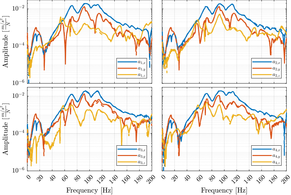
The comparison is made for the 4 accelerometers fixed on the micro-hexapod (Figure ref:fig:modal_comp_acc_solid_body_frf). The original frequency response functions and those computed from the CoM responses match well in the frequency range of interest. Similar results were obtained for the other solid bodies, indicating that the solid body assumption is valid and that a multi-body model can be used to represent the dynamics of the micro-station. This also validates the reduction in the number of degrees of freedom from 69 (23 accelerometers with each 3 acrshort:dof) to 36 (6 solid bodies with 6 acrshort:dof).

Comparaison of the original accelerometer response (solid curves) and the reconstructed response from the solid body response (dashed curves). Accelerometers 1 to 4 corresponding to the micro-hexapod are shown.

Modal Analysis

<<sec:modal_analysis>>

Introduction   ignore

The goal here is to extract the modal parameters describing the modes of the micro station being studied, namely, the natural frequencies and the modal damping (i.e. the eigenvalues) as well as the mode shapes (.i.e. the eigenvectors). This is performed from the acrshort:frf matrix previously extracted from the measurements.

In order to perform the modal parameter extraction, the order of the modal model has to be estimated (i.e. the number of modes in the frequency band of interest). This is achived using the acrfull:mif in section ref:ssec:modal_number_of_modes.

In section ref:ssec:modal_parameter_extraction, the modal parameter extraction is performed. The graphical display of the mode shapes can be computed from the modal model, which is quite quite useful for physical interpretation of the modes.

To validate the quality of the modal model, the full acrshort:frf matrix is computed from the modal model and compared to the initial measured acrshort:frf (section ref:ssec:modal_model_validity).

Number of modes determination

<<ssec:modal_number_of_modes>> The acrshort:mif is here applied to the $n\times p$ acrshort:frf matrix where $n$ is a relatively large number of measurement DOFs (here $n=69$) and $p$ is the number of excitation DOFs (here $p=3$).

The complex modal indication function is defined in equation eqref:eq:modal_cmif where the diagonal matrix $\Sigma$ is obtained from a acrlong:svd of the acrshort:frf matrix as shown in equation eqref:eq:modal_svd. \begin{equation} \label{eq:modal_cmif} [CMIF(ω)]_{p× p} = [Σ(ω)]_{p× n}^T [Σ(ω)]_{n× p}

\end{equation}

\begin{equation} \label{eq:modal_svd} [H(ω)]_{n× p} = [U(ω)]_{n× n} [Σ(ω)]_{n× p} [V(ω)]_{p× p}^H

\end{equation}

The acrshort:mif therefore yields to $p$ values that are also frequency dependent. A peak in the acrshort:mif plot indicates the presence of a mode. Repeated modes can also be detected when multiple singular values have peaks at the same frequency. The obtained acrshort:mif is shown on Figure ref:fig:modal_indication_function. A total of 16 modes were found between 0 and $200\,\text{Hz}$. The obtained natural frequencies and associated modal damping are summarized in Table ref:tab:modal_obtained_modes_freqs_damps.

%% Load frequency response matrix
load('frf_matrix.mat', 'freqs', 'frf');

%% Computation of the modal indication function
MIF = zeros(size(frf, 2), size(frf, 2), size(frf, 3));

for i = 1:length(freqs)
  [~,S,~] = svd(frf(:, :, i));
  MIF(:, :, i) = S'*S;
end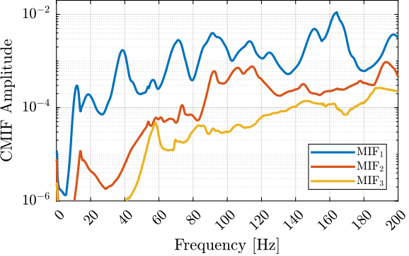

\hfill

Mode	Frequency	Damping
1	$11.9\,\text{Hz}$	$12.2\,\%$
2	$18.6\,\text{Hz}$	$11.7\,\%$
3	$37.8\,\text{Hz}$	$6.2\,\%$
4	$39.1\,\text{Hz}$	$2.8\,\%$
5	$56.3\,\text{Hz}$	$2.8\,\%$
6	$69.8\,\text{Hz}$	$4.3\,\%$
7	$72.5\,\text{Hz}$	$1.3\,\%$
8	$84.8\,\text{Hz}$	$3.7\,\%$
9	$91.3\,\text{Hz}$	$2.9\,\%$
10	$105.5\,\text{Hz}$	$3.2\,\%$
11	$106.6\,\text{Hz}$	$1.6\,\%$
12	$112.7\,\text{Hz}$	$3.1\,\%$
13	$124.2\,\text{Hz}$	$2.8\,\%$
14	$145.3\,\text{Hz}$	$1.3\,\%$
15	$150.5\,\text{Hz}$	$2.4\,\%$
16	$165.4\,\text{Hz}$	$1.4\,\%$

Modal parameter extraction

<<ssec:modal_parameter_extraction>>

Generally, modal identification consists of curve-fitting a theoretical expression to the actual measured acrshort:frf data. However, there are multiple levels of complexity, from fitting of a single resonance, to fitting a complete curve encompassing several resonances and working on a set of many acrshort:frf plots all obtained from the same structure.

Here, the last method is used because it provides a unique and consistent model. It takes into account the fact that the properties of all individual curves are related by being from the same structure: all acrshort:frf plots on a given structure should indicate the same values for the natural frequencies and damping factor of each mode.

From the obtained modal parameters, the mode shapes are computed and can be displayed in the form of animations (three mode shapes are shown in Figure ref:fig:modal_mode_animations).

Three obtained mode shape animations

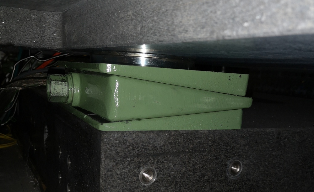
These animations are useful for visually obtaining a better understanding of the system's dynamic behavior. For instance, the mode shape of the first mode at $11\,\text{Hz}$ (figure ref:fig:modal_mode1_animation) indicates an issue with the lower granite. It turns out that four Airloc Levelers are used to level the lower granite (figure ref:fig:modal_airloc). These are difficult to adjust and can lead to a situation in which the granite is only supported by two of them; therefore, it has a low frequency "tilt mode". The levelers were then better adjusted.

The modal parameter extraction is made using a proprietary software⁵. For each mode $r$ (from $1$ to the number of considered modes $m=16$), it outputs the frequency $\omega_r$, the damping ratio $\xi_r$, the eigenvectors $\{\phi_{r}\}$ (vector of complex numbers with a size equal to the number of measured acrshort:dof $n=69$, see equation eqref:eq:modal_eigenvector) and a scaling factor $a_r$.

\begin{equation}\label{eq:modal_eigenvector} \{ɸ_i\} = \begin{Bmatrix} \phi_{i, 1_x} & \phi_{i, 1_y} & \phi_{i, 1_z} & \phi_{i, 2_x} & \dots & \phi_{i, 23_z} \end{Bmatrix}^T

\end{equation}

The eigenvalues $s_r$ and $s_r^*$ can then be computed from equation eqref:eq:modal_eigenvalues.

\begin{equation}\label{eq:modal_eigenvalues} s_r = ω_r (-ξ_r + i \sqrt{1 - ξ_r^2}), \quad s_r^* = ω_r (-ξ_r - i \sqrt{1 - ξ_r^2})

\end{equation}

Verification of the modal model validity

<<ssec:modal_model_validity>>

To check the validity of the modal model, the complete $n \times n$ acrshort:frf matrix $\mathbf{H}_{\text{syn}}$ is first synthesized from the modal parameters. Then, the elements of this acrshort:frf matrix $\mathbf{H}_{\text{syn}}$ that were already measured can be compared to the measured acrshort:frf matrix $\mathbf{H}$.

In order to synthesize the full acrshort:frf matrix, the eigenvectors $\phi_r$ are first organized in matrix from as shown in equation eqref:eq:modal_eigvector_matrix. \begin{equation}\label{eq:modal_eigvector_matrix} Φ = \begin{bmatrix} & & & & &\\ \phi_1 & \dots & \phi_N & \phi_1^* & \dots & \phi_N^* \\ & & & & & \end{bmatrix}_{n × 2m}

\end{equation}

The full acrshort:frf matrix $\mathbf{H}_{\text{syn}}$ can be synthesize using eqref:eq:modal_synthesized_frf.

\begin{equation}\label{eq:modal_synthesized_frf} [\mathbf{H}_{\text{syn}}(ω)]_{n× n} = [Φ]_n×2m [\mathbf{H}_{\text{mod}}(ω)]_2m×2m [Φ]_{2m× n}^T

\end{equation}

With $\mathbf{H}_{\text{mod}}(\omega)$ a diagonal matrix representing the response of the different modes eqref:eq:modal_modal_resp. \begin{equation}\label{eq:modal_modal_resp} \mathbf{H}_{\text{mod}}(ω) = \text{diag}≤ft(\frac{1}{a_1 (jω - s_1)},\ …,\ \frac{1}{a_m (jω - s_m)}, \frac{1}{a_1^* (jω - s_1^*)},\ …,\ \frac{1}{a_m^* (jω - s_m^*)} \right)_{2m× 2m}

\end{equation}

%% Load modal parameters
shapes_m = readtable('mat/mode_shapes.txt',              'ReadVariableNames', false);  % [Sign / Real / Imag]
freqs_m  = table2array(readtable('mat/mode_freqs.txt',   'ReadVariableNames', false)); % in [Hz]
damps_m  = table2array(readtable('mat/mode_damps.txt',   'ReadVariableNames', false)); % in [%]
modal_a  = table2array(readtable('mat/mode_modal_a.txt', 'ReadVariableNames', false)); % [Real / Imag]
modal_b  = table2array(readtable('mat/mode_modal_b.txt', 'ReadVariableNames', false)); % [Real / Imag]

%% Guess the number of modes identified from the length of the imported data.
acc_n = 23; % Number of accelerometers
dir_n = 3; % Number of directions
dirs = 'XYZ';

mod_n = size(shapes_m,1)/acc_n/dir_n; % Number of modes

%% Mode shapes are split into 3 parts (direction plus sign, real part and imaginary part)
% we aggregate them into one array of complex numbers
T_sign = table2array(shapes_m(:, 1));
T_real = table2array(shapes_m(:, 2));
T_imag = table2array(shapes_m(:, 3));

mode_shapes = zeros(mod_n, dir_n, acc_n);

for mod_i = 1:mod_n
  for acc_i = 1:acc_n
    % Get the correct section of the signs
    T = T_sign(acc_n*dir_n*(mod_i-1)+1:acc_n*dir_n*mod_i);
    for dir_i = 1:dir_n
      % Get the line corresponding to the sensor
      i = find(contains(T, sprintf('%i%s',acc_i, dirs(dir_i))), 1, 'first')+acc_n*dir_n*(mod_i-1);
      mode_shapes(mod_i, dir_i, acc_i) = str2num([T_sign{i}(end-1), '1'])*complex(T_real(i),T_imag(i));
    end
  end
end

%% Create the eigenvalue and eigenvector matrices
eigen_val_M = diag(2*pi*freqs_m.*(-damps_m/100 + j*sqrt(1 - (damps_m/100).^2))); % Lambda = diagonal matrix
eigen_vec_M = reshape(mode_shapes, [mod_n, acc_n*dir_n]).'; % Phi, vecnorm(eigen_vec_M) = 1

% Add complex conjugate eigenvalues and eigenvectors
eigen_val_ext_M = blkdiag(eigen_val_M, conj(eigen_val_M));
eigen_vec_ext_M = [eigen_vec_M, conj(eigen_vec_M)];

%% "Modal A" and "Modal B" matrices
modal_a_M = diag(complex(modal_a(:, 1), modal_a(:, 2)));
modal_b_M = diag(complex(modal_b(:, 1), modal_b(:, 2)));

modal_a_ext_M = blkdiag(modal_a_M, conj(modal_a_M));
modal_b_ext_M = blkdiag(modal_b_M, conj(modal_b_M));

%% Synthesize the full FRF matrix from the modal model
Hsyn = zeros(acc_n*dir_n, acc_n*dir_n, length(freqs));

for i = 1:length(freqs)
  Hsyn(:, :, i) = eigen_vec_ext_M*diag(1./(diag(modal_a_ext_M).*(j*2*pi*freqs(i) - diag(eigen_val_ext_M))))*eigen_vec_ext_M.';
end

%% Derivate two times to to have the acceleration response
for i = 1:size(Hsyn, 1)
  Hsyn(i, :, :) = squeeze(Hsyn(i, :, :)).*(j*2*pi*freqs).^2;
end

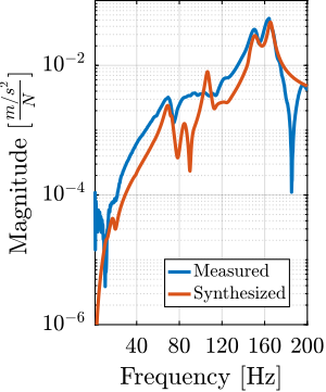
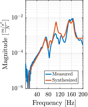
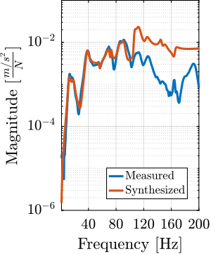
A comparison between original measured frequency response functions and synthesized ones from the modal model is presented in Figure ref:fig:modal_comp_acc_frf_modal. Whether the obtained match is good or bad is quite arbitrary. However, the modal model seems to be able to represent the coupling between different nodes and different directions, which is quite important from a control perspective. This can be seen in Figure ref:fig:modal_comp_acc_frf_modal_3 that shows the frequency response function from the force applied on node 11 (i.e. on the translation stage) in the $y$ direction to the measured acceleration at node $2$ (i.e. at the top of the micro-hexapod) in the $x$ direction.

Conclusion

<<sec:modal_conclusion>>

In this study, a modal analysis of the micro-station was performed. Thanks to an adequate choice of instrumentation and proper set of measurements, high quality frequency response functions can be obtained. The obtained frequency response functions indicate that the dynamics of the micro-station are complex, which is expected from a heavy stack stage architecture. It shows a lot of coupling between stages and different directions, and many modes.

By measuring 12 degrees of freedom on each "stage", it could be verified that in the frequency range of interest, each stage behaved as a rigid body. This confirms that a multi-body model can be used to properly model the micro-station.

Although a lot of effort was put into this experimental modal analysis of the micro-station, it was difficult to obtain an accurate modal model. However, the measurements are useful for tuning the parameters of the micro-station multi-body model.

Bibliography   ignore

Glossary   ignore

printglossaries:

Footnotes

⁴As this matrix is in general non-square, the Moore–Penrose inverse can be used instead. ⁵NVGate software from OROS company. ³OROS OR36. 24bits signal-delta ADC. ²Kistler 9722A2000. Sensitivity of $2.3\,mV/N$ and measurement range of $2\,kN$ ¹PCB 356B18. Sensitivity is $1\,V/g$, measurement range is $\pm 5\,g$ and bandwidth is $0.5$ to $5\,\text{kHz}$.

---