Identification

1. Some notes about the Simscape Model
2. Compare with measurements at the CoM of each element
3. Obtained Compliance of the Micro-Station
- 3.1. Initialization
4. Conclusion

The goal here is to tune the Simscape model of the station in order to have a good dynamical representation of the real system.

In order to do so, we reproduce the Modal Analysis done on the station using the Simscape model.

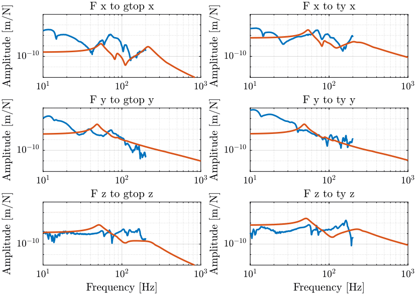
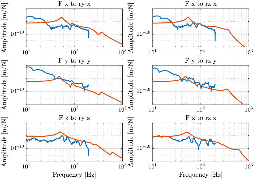
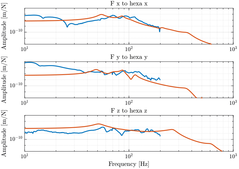
We can then compare the measured Frequency Response Functions with the identified dynamics of the model.

Finally, this should help to tune the parameters of the model such that the dynamics is closer to the measured FRF.

1 Some notes about the Simscape Model

The Simscape Model of the micro-station consists of several solid bodies:

Bottom Granite
Top Granite
Translation Stage
Tilt Stage
Spindle
Hexapod

Each solid body has some characteristics: Center of Mass, mass, moment of inertia, etc… These parameters are automatically computed from the geometry and from the density of the materials.

Then, the solid bodies are connected with springs and dampers. Some of the springs and dampers values can be estimated from the joints/stages specifications, however, we here prefer to tune these values based on the measurements.

2 Compare with measurements at the CoM of each element

2.1 Prepare the Simulation

We load the configuration.

  load('mat/conf_simulink.mat');

We set a small StopTime.

  set_param(conf_simulink, 'StopTime', '0.5');

We initialize all the stages.

  initializeGround(      'type', 'rigid');
  initializeGranite(     'type', 'modal-analysis');
  initializeTy(          'type', 'modal-analysis');
  initializeRy(          'type', 'modal-analysis');
  initializeRz(          'type', 'modal-analysis');
  initializeMicroHexapod('type', 'modal-analysis');
  initializeAxisc(       'type', 'flexible');

  initializeMirror(      'type', 'none');
  initializeNanoHexapod( 'type', 'none');
  initializeSample(      'type', 'none');

  initializeController(  'type', 'open-loop');

  initializeLoggingConfiguration('log', 'none');

  initializeReferences();
  initializeDisturbances('enable', false);

2.2 Estimate the position of the CoM of each solid and compare with the one took for the Measurement Analysis

Thanks to the Inertia Sensor simscape block, it is possible to estimate the position of the Center of Mass of a solid body with respect to a defined frame.

  sim('nass_model')

The results are shown in the table 1.

Table 1: Center of Mass of each solid body as defined in Simscape
	granite bot	granite top	ty	ry	rz	hexa
X [mm]	52.4	51.7	0.9	-0.1	0.0	-0.0
Y [mm]	190.4	263.2	0.7	5.2	-0.0	0.1
Z [mm]	-1200.0	-777.1	-598.9	-627.7	-643.2	-317.1

We can compare the obtained center of mass (table 1) with the one used for the Modal Analysis shown in table 2.

Table 2: Estimated Center of Mass of each solid body using Solidworks
	granite bot	granite top	ty	ry	rz	hexa
X [mm]	45	52	0	0	0	-4
Y [mm]	144	258	14	-5	0	6
Z [mm]	-1251	-778	-600	-628	-580	-319

The results are quite similar. The differences can be explained by some differences in the chosen density of the materials or by the fact that not exactly all the same elements have been chosen for each stage.

For instance, on simscape, the fixed part of the translation stage counts for the top granite solid body. However, in SolidWorks, this has probably not be included with the top granite.

2.3 Create a frame at the CoM of each solid body

Now we use one inertiasensor block connected on each solid body that measured the center of mass of this solid with respect to the same connected frame.

We do that in order to position an accelerometer on the Simscape model at this particular point.

  open('identification/matlab/sim_micro_station_com_estimation.slx')

  sim('sim_micro_station_com_estimation')

	granite bot	granite top	ty	ry	rz	hexa
X [mm]	0.0	51.7	0.9	-0.1	0.0	-0.0
Y [mm]	0.0	753.2	0.7	5.2	-0.0	0.1
Z [mm]	-250.0	22.9	-17.1	-146.5	-23.2	-47.1

We now same this for further use:

  granite_bot_com = granite_bot_com.Data(end, :)';
  granite_top_com = granite_top_com.Data(end, :)';
  ty_com = ty_com.Data(end, :)';
  ry_com = ry_com.Data(end, :)';
  rz_com = rz_com.Data(end, :)';
  hexa_com = hexa_com.Data(end, :)';

  save('./mat/solids_com.mat', 'granite_bot_com', 'granite_top_com', 'ty_com', 'ry_com', 'rz_com', 'hexa_com');

Then, we use the obtained results to add a rigidTransform block in order to create a new frame at the center of mass of each solid body.

2.4 Identification of the dynamics of the Simscape Model

We now use a new Simscape Model where 6DoF inertial sensors are located at the Center of Mass of each solid body.

  % load('mat/solids_com.mat', 'granite_bot_com', 'granite_top_com', 'ty_com', 'ry_com', 'rz_com', 'hexa_com');

  open('nass_model.slx')

We use the linearize function in order to estimate the dynamics from forces applied on the Translation stage at the same position used for the real modal analysis to the inertial sensors.

  %% Options for Linearized
  options = linearizeOptions;
  options.SampleTime = 0;

  %% Name of the Simulink File
  mdl = 'nass_model';

  %% Input/Output definition
  clear io; io_i = 1;
  io(io_i) = linio([mdl, '/Micro-Station/Translation Stage/Modal Analysis/F_hammer'],          1, 'openinput');  io_i = io_i + 1;
  io(io_i) = linio([mdl, '/Micro-Station/Granite/Modal Analysis/accelerometer'],               1, 'openoutput'); io_i = io_i + 1;
  io(io_i) = linio([mdl, '/Micro-Station/Translation Stage/Modal Analysis/accelerometer'],     1, 'openoutput'); io_i = io_i + 1;
  io(io_i) = linio([mdl, '/Micro-Station/Tilt Stage/Modal Analysis/accelerometer'],            1, 'openoutput'); io_i = io_i + 1;
  io(io_i) = linio([mdl, '/Micro-Station/Spindle/Modal Analysis/accelerometer'],               1, 'openoutput'); io_i = io_i + 1;
  io(io_i) = linio([mdl, '/Micro-Station/Micro Hexapod/Modal Analysis/accelerometer'],         1, 'openoutput'); io_i = io_i + 1;

  % Run the linearization
  G_ms = linearize(mdl, io, 0);

  %% Input/Output definition
  G_ms.InputName  = {'Fx', 'Fy', 'Fz'};
  G_ms.OutputName = {'gtop_x', 'gtop_y', 'gtop_z', 'gtop_rx', 'gtop_ry', 'gtop_rz', ...
                     'ty_x', 'ty_y', 'ty_z', 'ty_rx', 'ty_ry', 'ty_rz', ...
                     'ry_x', 'ry_y', 'ry_z', 'ry_rx', 'ry_ry', 'ry_rz', ...
                     'rz_x', 'rz_y', 'rz_z', 'rz_rx', 'rz_ry', 'rz_rz', ...
                     'hexa_x', 'hexa_y', 'hexa_z', 'hexa_rx', 'hexa_ry', 'hexa_rz'};

The output of G_ms is the acceleration of each solid body. In order to obtain a displacement, we divide the obtained transfer function by \(1/s^{2}\);

  G_ms = G_ms/s^2;

2.5 Compare with measurements

We now load the Frequency Response Functions measurements during the Modal Analysis (accessible here).

  load('../meas/modal-analysis/mat/frf_coh_matrices.mat', 'freqs');
  load('../meas/modal-analysis/mat/frf_com.mat', 'FRFs_CoM');

We then compare the measurements with the identified transfer functions using the Simscape Model.

Figure 1: caption (png, pdf)

Figure 2: caption (png, pdf)

Figure 3: caption (png, pdf)

3 Obtained Compliance of the Micro-Station

3.1 Initialization

We initialize all the stages with the default parameters.

  initializeGround();
  initializeGranite();
  initializeTy();
  initializeRy();
  initializeRz();
  initializeMicroHexapod('type', 'compliance');

We put nothing on top of the micro-hexapod.

  initializeAxisc('type', 'none');
  initializeMirror('type', 'none');
  initializeNanoHexapod('type', 'none');
  initializeSample('type', 'none');

  initializeReferences();
  initializeDisturbances();
  initializeController();
  initializeSimscapeConfiguration();
  initializeLoggingConfiguration();

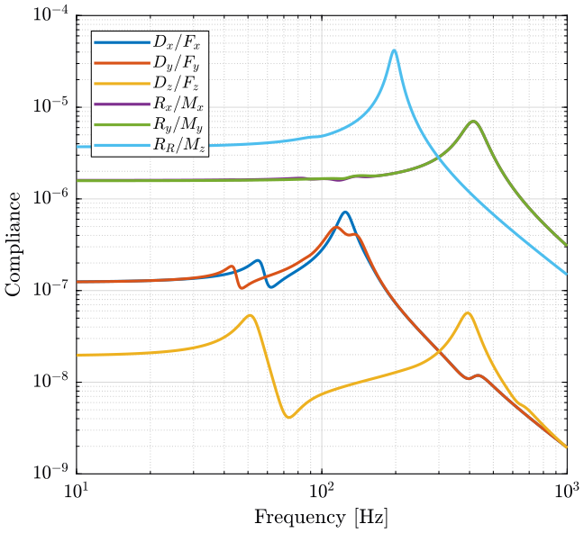
And we identify the dynamics from forces/torques applied on the micro-hexapod top platform to the motion of the micro-hexapod top platform at the same point.

The obtained compliance is shown in Figure 4.

  %% Name of the Simulink File
  mdl = 'nass_model';

  %% Input/Output definition
  clear io; io_i = 1;
  io(io_i) = linio([mdl, '/Micro-Station/Micro Hexapod/Compliance/Fm'], 1, 'openinput');       io_i = io_i + 1; % Direct Forces/Torques applied on the micro-hexapod top platform
  io(io_i) = linio([mdl, '/Micro-Station/Micro Hexapod/Compliance/Dm'], 1, 'output'); io_i = io_i + 1; % Absolute displacement of the top platform

  %% Run the linearization
  Gm = linearize(mdl, io, 0);
  Gm.InputName  = {'Fmx', 'Fmy', 'Fmz', 'Mmx', 'Mmy', 'Mmz'};
  Gm.OutputName = {'Dx', 'Dy', 'Dz', 'Drx', 'Dry', 'Drz'};

  save('../meas/micro-station-compliance/mat/model.mat', 'Gm');

Figure 4: Obtained compliance of the Micro-Station (png, pdf)

4 Conclusion

For such a complex system, we believe that the Simscape Model represents the dynamics of the system with enough fidelity.