Determination of the optimal nano-hexapod’s stiffness for reducing the effect of disturbances
Table of Contents
In this document is studied how the stiffness of the nano-hexapod will impact the effect of disturbances on the position error of the sample.
It is divided in the following sections:
- Section 1: the disturbances are listed and their Power Spectral Densities (PSD) are shown
- Section 2: the transfer functions from disturbances to the position error of the sample are computed for a wide range of nano-hexapod stiffnesses
- Section 3:
- Section 4: from both the PSD of the disturbances and the transfer function from disturbances to sample’s position errors, we compute the resulting PSD and Cumulative Amplitude Spectrum (CAS)
- Section 5: from a simplistic model is computed the required control bandwidth to reduce the position error to acceptable values
1 Disturbances
The main disturbances considered here are:
- \(D_w\): Ground displacement in the \(x\), \(y\) and \(z\) directions
- \(F_{ty}\): Forces applied by the Translation stage in the \(x\) and \(z\) directions
- \(F_{rz}\): Forces applied by the Spindle in the \(z\) direction
- \(F_d\): Direct forces applied at the center of mass of the Payload
The level of these disturbances has been identified form experiments which are detailed in this document.
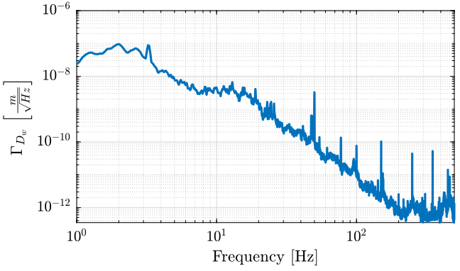
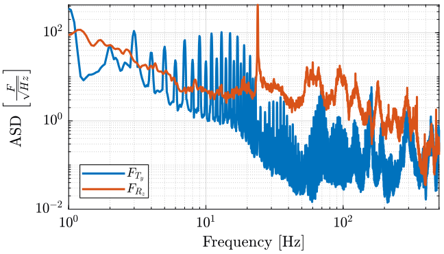
The measured Amplitude Spectral Densities (ASD) of these forces are shown in Figures 1 and 2.
In this study, the expected frequency content of the direct forces applied to the payload is not considered.
2 Effect of disturbances on the position error
In this section, we use the Simscape model to identify the transfer function from disturbances to the position error of the sample. We do that for a wide range of nano-hexapod stiffnesses and we compare the obtained results.
2.1 Initialization
We initialize all the stages with the default parameters.
initializeGround();
initializeGranite();
initializeTy();
initializeRy();
initializeRz();
initializeMicroHexapod();
initializeAxisc();
initializeMirror();
We use a sample mass of 10kg.
initializeSample('mass', 10);
We include gravity, and we use no controller.
initializeSimscapeConfiguration('gravity', true);
initializeController();
initializeDisturbances('enable', false);
initializeLoggingConfiguration('log', 'none');
2.2 Identification
The considered inputs are:
Dwx: Ground displacement in the \(x\) directionDwy: Ground displacement in the \(y\) directionDwz: Ground displacement in the \(z\) directionFty_x: Forces applied by the Translation stage in the \(x\) directionFty_z: Forces applied by the Translation stage in the \(z\) directionFrz_z: Forces applied by the Spindle in the \(z\) directionFd: Direct forces applied at the center of mass of the Payload
The outputs are Ex, Ey, Ez, Erx, Ery, Erz which are the 3 positions and 3 orientations errors of the sample.
We initialize the set of the nano-hexapod stiffnesses, and for each of them, we identify the dynamics from defined inputs to defined outputs.
Ks = logspace(3,9,7); % [N/m]
2.3 Sensitivity to Stages vibration (Filtering)
The sensitivity the stage vibrations are displayed:
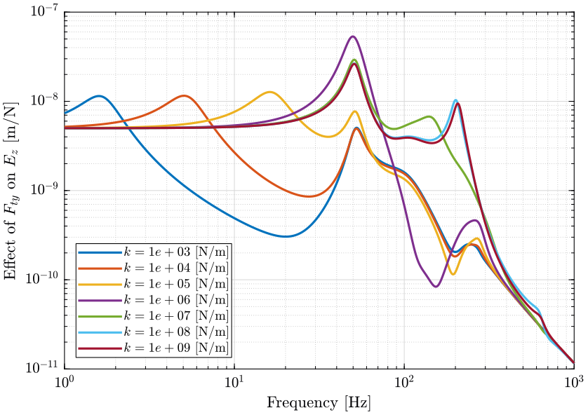
- Figure 3: sensitivity to vertical spindle vibrations
- Figure 4: sensitivity to vertical translation stage vibrations
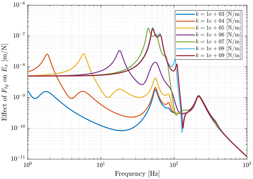
- Figure 5: sensitivity to horizontal (x) translation stage vibrations
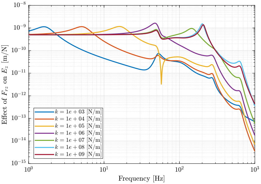
Figure 3: Sensitivity to Spindle vertical motion error (\(F_{rz}\)) to the vertical error position of the sample (\(E_z\)) (png, pdf)
2.4 Effect of Ground motion (Transmissibility).
2.5 Direct Forces (Compliance).
2.6 Conclusion
Reducing the nano-hexapod stiffness generally lowers the sensitivity to stages vibration but increases the sensitivity to ground motion and direct forces.
In order to conclude on the optimal stiffness that will yield the smallest sample vibration, one has to include the level of disturbances. This is done in Section 4.
3 Effect of granite stiffness
In this section, we wish to see if a soft granite suspension could help in reducing the effect of disturbances on the position error of the sample.
3.1 Analytical Analysis
3.1.1 Simple mass-spring-damper model
Let’s consider the system shown in Figure 8 consisting of two stacked mass-spring-damper systems. The bottom one represents the granite, and the top one all the positioning stages. We want the smallest stage “deformation” \(d = x^\prime - x\) due to ground motion \(w\).
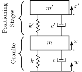
Figure 8: Mass Spring Damper system consisting of a granite and a positioning stage
If we write the equation of motion of the system in Figure 8, we obtain:
\begin{align} m^\prime s^2 x^\prime &= (c^\prime s + k^\prime) (x - x^\prime) \\ ms^2 x &= (c^\prime s + k^\prime) (x^\prime - x) + (cs + k) (w - x) \end{align}If we note \(d = x^\prime - x\), we obtain:
\begin{equation} \frac{d}{w} = \frac{-m^\prime s^2 (cs + k)}{ (m^\prime s^2 + c^\prime s + k^\prime) (ms^2 + cs + k) + m^\prime s^2(c^\prime s + k^\prime)} \end{equation}3.1.2 General Case
Let’s now considering a general positioning stage defined by:
- \(G^\prime(s) = \frac{F}{x}\): its mechanical “impedance”
- \(D^\prime(s) = \frac{d}{x}\): its “deformation” transfer function
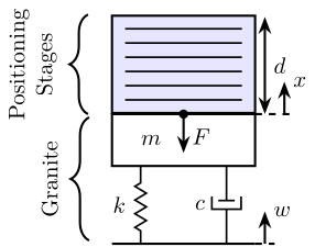
Figure 9: Mass Spring Damper representing the granite and a general representation of positioning stages
The equation of motion are:
\begin{align} ms^2 x &= (cs + k) (x - w) - F \\ F &= G^\prime(s) x \\ d &= D^\prime(s) x \end{align}where:
- \(F\) is the force applied by the position stages on the granite mass
We can express \(d\) as a function of \(w\):
\begin{equation} \frac{d}{w} = \frac{D^\prime(s) (cs + k)}{ms^2 + cs + k + G^\prime(s)} \end{equation}This is the transfer function that we would like to minimize.
Let’s verify this formula for a simple mass/spring/damper positioning stage. In that case, we have:
\begin{align*} D^\prime(s) &= \frac{d}{x} = \frac{- m^\prime s^2}{m^\prime s^2 + c^\prime s + k^\prime} \\ G^\prime(s) &= \frac{F}{x} = \frac{m^\prime s^2(c^\prime s + k)}{m^\prime s^2 + c^\prime s + k^\prime} \end{align*}And finally:
\begin{equation} \frac{d}{w} = \frac{-m^\prime s^2 (cs + k)}{ (m^\prime s^2 + c^\prime s + k^\prime) (ms^2 + cs + k) + m^\prime s^2(c^\prime s + k^\prime)} \end{equation}which is the same as the previously derived equation.
3.2 Soft Granite
Let’s initialize a soft granite and see how the sensitivity to disturbances will change.
initializeGranite('K', 5e5*ones(3,1), 'C', 5e3*ones(3,1));
3.3 Effect of the Granite transfer function
From Figure 10, we can see that having a “soft” granite suspension greatly lowers the sensitivity to ground motion. The sensitivity is indeed lowered starting from the resonance of the granite on its soft suspension (few Hz here).
From Figures 11 and 12, we see that the change of granite suspension does not change a lot the sensitivity to both direct forces and stage vibrations.
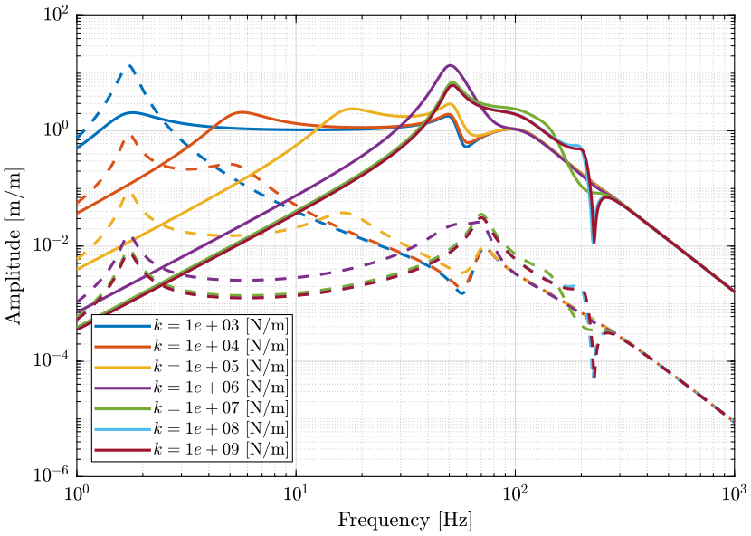
Figure 10: Change of sensibility to Ground motion when using a stiff Granite (solid curves) and a soft Granite (dashed curves) (png, pdf)
3.4 Conclusion
Having a soft granite suspension greatly decreases the sensitivity the ground motion. Also, it does not affect much the sensitivity to stage vibration and direct forces. Thus the level of sample vibration can be reduced by using a soft granite suspension if it is found that ground motion is the limiting factor.
4 Open Loop Budget Error
Now that the frequency content of disturbances have been estimated (Section 1) and the transfer functions from disturbances to the position error of the sample have been identified (Section 2), we can compute the level of sample vibration due to the disturbances.
We then can conclude and the nano-hexapod stiffness that will lower the sample position error.
4.1 Noise Budgeting - Theory
Let’s consider Figure 13 there \(G_d(s)\) is the transfer function from a signal \(d\) (the perturbation) to a signal \(y\) (the sample’s position error).

Figure 13: Signal \(d\) going through and LTI transfer function \(G_d(s)\) to give a signal \(y\)
We can compute the Power Spectral Density (PSD) of signal \(y\) from the PSD of \(d\) and the norm of \(G_d(s)\):
\begin{equation} S_{y}(\omega) = \left|G_d(j\omega)\right|^2 S_{d}(\omega) \label{eq:psd_transfer_function} \end{equation}If we now consider multiple disturbances \(d_1, \dots, d_n\) as shown in Figure 14, we have that:
\begin{equation} S_{y}(\omega) = \left|G_{d_1}(j\omega)\right|^2 S_{d_1}(\omega) + \dots + \left|G_{d_n}(j\omega)\right|^2 S_{d_n}(\omega) \label{eq:sum_psd} \end{equation}Sometimes, we prefer to compute the Amplitude Spectral Density (ASD) which is related to the PSD by: \[ \Gamma_y(\omega) = \sqrt{S_y(\omega)} \]
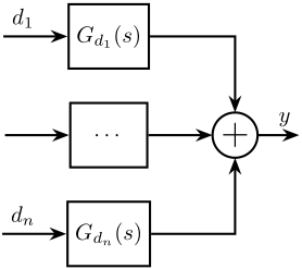
Figure 14: Block diagram showing and output \(y\) resulting from the addition of multiple perturbations \(d_i\)
The Cumulative Power Spectrum (CPS) is here defined as:
\begin{equation} \Phi_y(\omega) = \int_\omega^\infty S_y(\nu) d\nu \end{equation}And the Cumulative Amplitude Spectrum (CAS):
\begin{equation} \Psi(\omega) = \sqrt{\Phi(\omega)} = \sqrt{\int_\omega^\infty S_y(\nu) d\nu} \end{equation}The CAS evaluation for all frequency corresponds to the rms value of the considered quantity: \[ y_{\text{rms}} = \Psi(\omega = 0) = \sqrt{\int_0^\infty S_y(\nu) d\nu} \]
4.2 Power Spectral Densities
We compute the effect of perturbations on the motion error thanks to Eq. \eqref{eq:psd_transfer_function}.
The result is shown in:
- Figure 15: PSD of the vertical sample’s motion error due to vertical ground motion
- Figure 16: PSD of the vertical sample’s motion error due to vertical vibrations of the Spindle

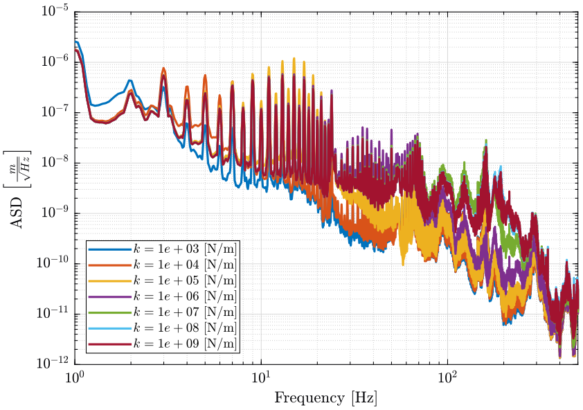
Figure 15: Amplitude Spectral Density of the Sample vertical position error due to Ground motion for multiple nano-hexapod stiffnesses (png, pdf)

Figure 16: Amplitude Spectral Density of the Sample vertical position error due to Vertical vibration of the Spindle for multiple nano-hexapod stiffnesses (png, pdf)
We compute the effect of all perturbations on the vertical position error using Eq. \eqref{eq:sum_psd} and the resulting PSD is shown in Figure 17.
4.3 Cumulative Amplitude Spectrum
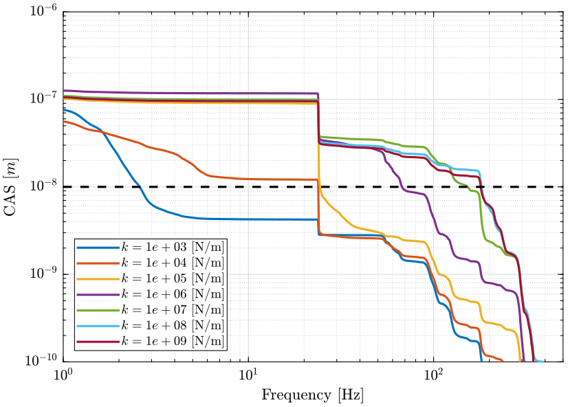
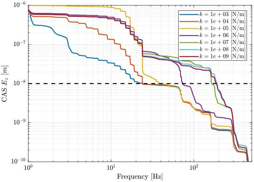
Similarly, the Cumulative Amplitude Spectrum of the sample vibrations are shown:
- Figure 18: due to vertical ground motion
- Figure 19: due to vertical vibrations of the Spindle
- Figure 20: due to all considered perturbations
The black dashed line corresponds to the performance objective of a sample vibration equal to \(10\ nm [rms]\).
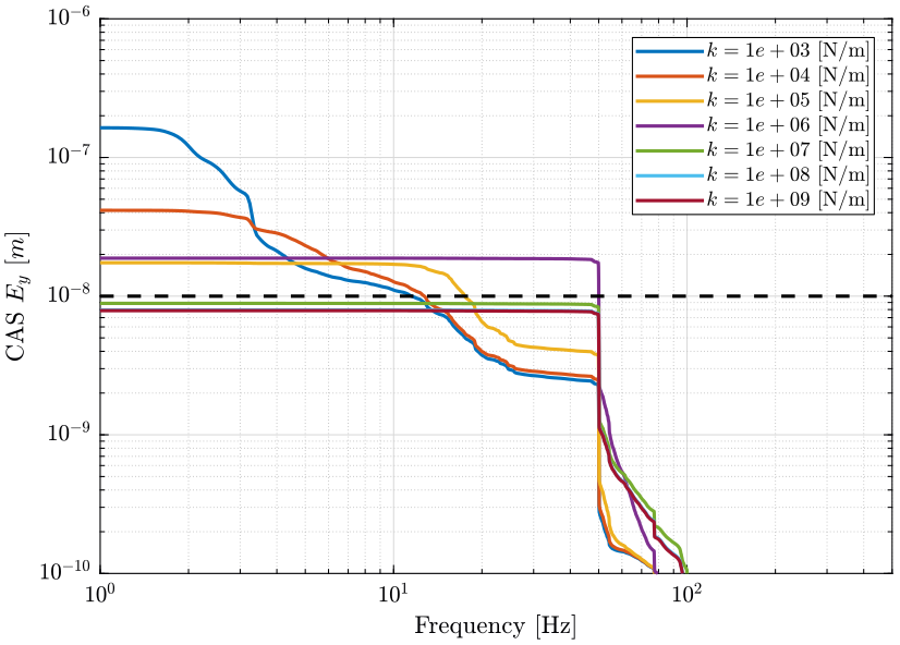
Figure 18: Cumulative Amplitude Spectrum of the Sample vertical position error due to Ground motion for multiple nano-hexapod stiffnesses (png, pdf)
4.4 Conclusion
From Figure 20, we can see that a soft nano-hexapod \(k<10^6\ [N/m]\) significantly reduces the effect of perturbations from 20Hz to 300Hz.
5 Closed Loop Budget Error
From the total open-loop power spectral density of the sample’s motion error, we can estimate what is the required control bandwidth for the sample’s motion error to be reduced down to \(10nm\).
5.1 Approximation of the effect of feedback on the motion error
Let’s consider Figure 21 where a controller \(K\) is used to reduce the effect of the disturbance \(d\) on the position error \(y\).
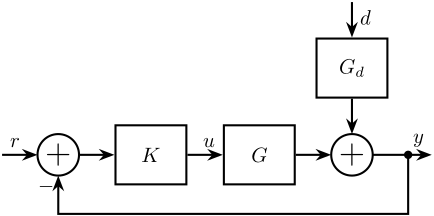
Figure 21: Feedback System
The reduction of the impact of \(d\) on \(y\) thanks to feedback is described by the following equation:
\begin{equation} \frac{y}{d} = \frac{G_d}{1 + KG} \end{equation}The transfer functions corresponding to \(G_d\) are those identified in Section 2.
As a first approximation, we can consider that the controller \(K\) is designed in such a way that the loop gain \(KG\) is a pure integrator: \[ L_1(s) = K_1(s) G(s) = \frac{\omega_c}{s} \] where \(\omega_c\) is the crossover frequency.
We may then consider another controller in such a way that the loop gain corresponds to a double integrator with a lead centered with the crossover frequency \(\omega_c\): \[ L_2(s) = K_2(s) G(s) = \left( \frac{\omega_c}{s} \right)^2 \cdot \frac{1 + \frac{s}{\omega_c/2}}{1 + \frac{s}{2\omega_c}} \]
In the next section, we see how the power spectral density of \(y\) is reduced as a function of the control bandwidth \(\omega_c\). This will help to determine what is the approximate control bandwidth required such that the rms value of \(y\) is below \(10nm\).
5.2 Reduction thanks to feedback - Required bandwidth
Let’s first see how does the Cumulative Amplitude Spectrum of the sample’s motion error is modified by the control.
In Figure 22 is shown the Cumulative Amplitude Spectrum of the sample’s motion error in Open-Loop and in Closed Loop for several control bandwidth (from 1Hz to 200Hz) and 4 different nano-hexapod stiffnesses. The controller used in this simulation is \(K_1\). The loop gain is then a pure integrator.
In Figure 23 is shown the expected RMS value of the sample’s position error as a function of the control bandwidth, both for \(K_1\) (left plot) and \(K_2\) (right plot). As expected, it is shown that \(K_2\) performs better than \(K_1\). This Figure tells us how much control bandwidth is required to attain a certain level of performance, and that for all the considered nano-hexapod stiffnesses.
The obtained required bandwidth (approximate upper and lower bounds) to obtained a sample’s motion error less than 10nm rms are gathered in Table 1.

Figure 22: Cumulative Amplitude Spectrum of the sample’s motion error in Open-Loop and in Closed Loop for several control bandwidth and 4 different nano-hexapod stiffnesses (png, pdf)

Figure 23: Expected RMS value of the sample’s motion error \(E_z\) as a function of the control bandwidth when using \(K_1\) and \(K_2\) (png, pdf)
| Nano-Hexapod stiffness [N/m] | 10^3 | 10^4 | 10^5 | 10^6 | 10^7 | 10^8 | 10^9 |
|---|---|---|---|---|---|---|---|
| Required wc with L1 [Hz] | 152 | 305 | 1000 | 870 | 933 | 870 | 870 |
| Required wc with L2 [Hz] | 57 | 66 | 152 | 152 | 248 | 266 | 248 |
6 Conclusion
From Figure 23 and Table 1, we can clearly see three different results depending on the nano-hexapod stiffness:
- For a soft nano-hexapod (\(k < 10^4\ [N/m]\)), the required bandwidth is \(\omega_c \approx 50-100\ Hz\)
- For a nano-hexapods with \(10^5 < k < 10^6\ [N/m]\), the required bandwidth is \(\omega_c \approx 150-300\ Hz\)
- For a stiff nano-hexapods (\(k > 10^7\ [N/m]\)), the required bandwidth is \(\omega_c \approx 250-500\ Hz\)
