Control of the NASS with Voice coil actuators

1. HAC-LAC + Cascade Control Topology
2. Other analysis

1 HAC-LAC + Cascade Control Topology

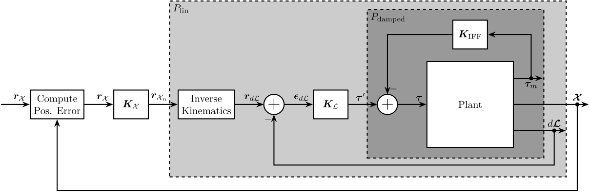
Figure 1: Cascaded Control consisting of (from inner to outer loop): IFF, Linearization Loop, Tracking Control in the frame of the Legs

1.1 Initialization

We initialize all the stages with the default parameters.

initializeGround();
initializeGranite();
initializeTy();
initializeRy();
initializeRz();
initializeMicroHexapod();
initializeAxisc();
initializeMirror();

The nano-hexapod is a voice coil based hexapod and the sample has a mass of 1kg.

initializeNanoHexapod('actuator', 'lorentz');
initializeSample('mass', 1);

We set the references that corresponds to a tomography experiment.

initializeReferences('Rz_type', 'rotating', 'Rz_period', 1);

initializeDisturbances();

initializeController('type', 'cascade-hac-lac');

initializeSimscapeConfiguration('gravity', true);

We log the signals.

initializeLoggingConfiguration('log', 'all');

Kp = tf(zeros(6));
Kl = tf(zeros(6));
Kiff = tf(zeros(6));

1.2 Low Authority Control - Integral Force Feedback \(\bm{K}_\text{IFF}\)

1.2.1 Identification

Let’s first identify the plant for the IFF controller.

%% Name of the Simulink File
mdl = 'nass_model';

%% Input/Output definition
clear io; io_i = 1;
io(io_i) = linio([mdl, '/Controller'],    1, 'openinput');               io_i = io_i + 1; % Actuator Inputs
io(io_i) = linio([mdl, '/Micro-Station'], 3, 'openoutput', [], 'Fnlm');  io_i = io_i + 1; % Force Sensors

%% Run the linearization
G_iff = linearize(mdl, io, 0);
G_iff.InputName  = {'Fnl1', 'Fnl2', 'Fnl3', 'Fnl4', 'Fnl5', 'Fnl6'};
G_iff.OutputName = {'Fnlm1', 'Fnlm2', 'Fnlm3', 'Fnlm4', 'Fnlm5', 'Fnlm6'};

1.2.2 Plant

The obtained plant for IFF is shown in Figure 2.

Figure 2: IFF Plant (png, pdf)

1.2.3 Root Locus

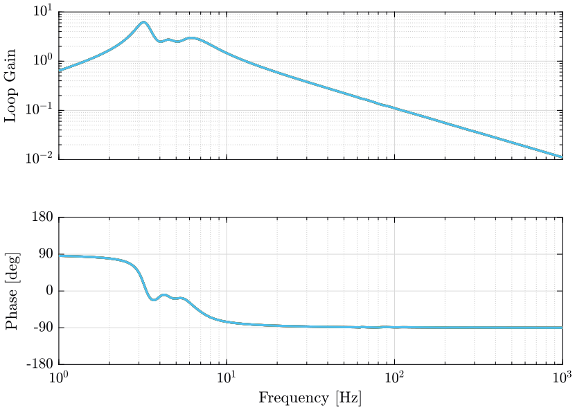
As seen in the root locus (Figure 3, no damping can be added to modes corresponding to the resonance of the micro-station.

However, critical damping can be achieve for the resonances of the nano-hexapod as shown in the zoomed part of the root (Figure 3, left part). The maximum damping is obtained for a control gain of \(\approx 70\).

Figure 3: Root Locus for the IFF control (png, pdf)

1.2.4 Controller and Loop Gain

We create the \(6 \times 6\) diagonal Integral Force Feedback controller. The obtained loop gain is shown in Figure 4.

Kiff = -70/s*eye(6);

Figure 4: Obtained Loop gain the IFF Control (png, pdf)

1.3 High Authority Control in the joint space - \(\bm{K}_\mathcal{L}\)

1.3.1 Identification of the damped plant

Let’s identify the dynamics from \(\bm{\tau}^\prime\) to \(d\bm{\mathcal{L}}\) as shown in Figure 1.

%% Name of the Simulink File
mdl = 'nass_model';

%% Input/Output definition
clear io; io_i = 1;
io(io_i) = linio([mdl, '/Controller'],    1, 'input');               io_i = io_i + 1; % Actuator Inputs
io(io_i) = linio([mdl, '/Micro-Station'], 3, 'output', [], 'Dnlm');  io_i = io_i + 1; % Leg Displacement

%% Run the linearization
Gl = linearize(mdl, io, 0);
Gl.InputName  = {'Fnl1', 'Fnl2', 'Fnl3', 'Fnl4', 'Fnl5', 'Fnl6'};
Gl.OutputName = {'Dnlm1', 'Dnlm2', 'Dnlm3', 'Dnlm4', 'Dnlm5', 'Dnlm6'};

There are some unstable poles in the Plant with very small imaginary parts. These unstable poles are probably not physical, and they disappear when taking the minimum realization of the plant.

isstable(Gl)
Gl = minreal(Gl);
isstable(Gl)

1.3.2 Obtained Plant

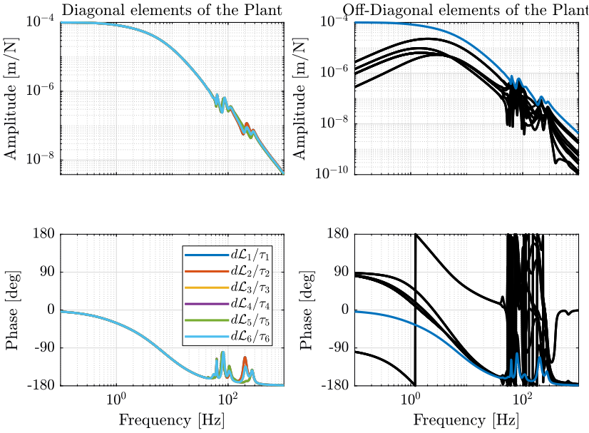
The obtained dynamics is shown in Figure 5.

Few things can be said on the dynamics:

the dynamics of the diagonal elements are almost all the same
the system is well decoupled below the resonances of the nano-hexapod (1Hz)
the dynamics of the diagonal elements are almost equivalent to a critically damped mass-spring-system with some spurious resonances above 50Hz corresponding to the resonances of the micro-station

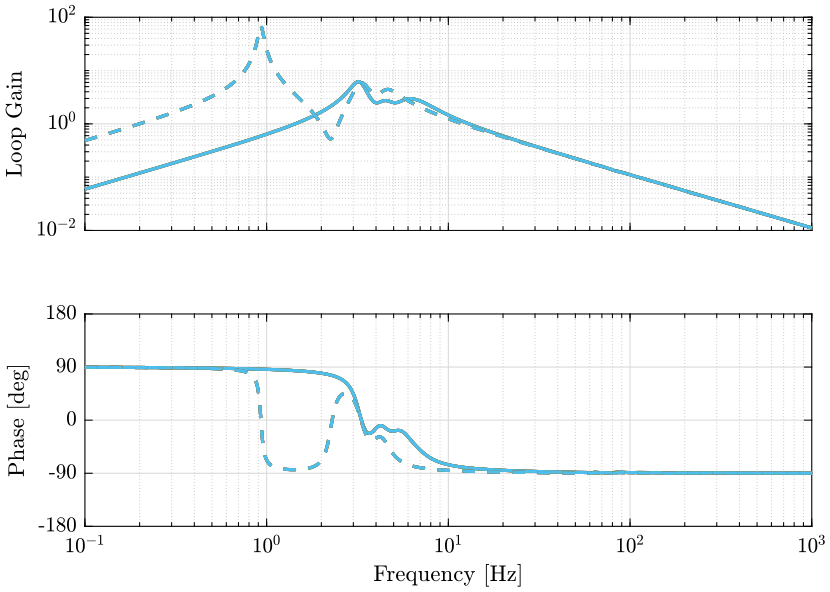
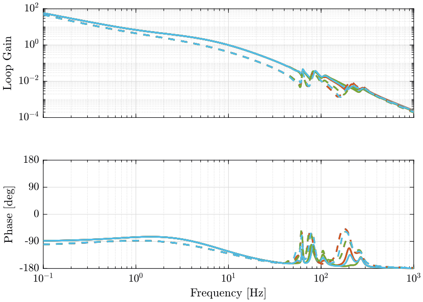
Figure 5: Plant for the High Authority Control in the Joint Space (png, pdf)

1.3.3 Controller Design and Loop Gain

As the plant is well decoupled, a diagonal plant is designed.

wc = 2*pi*10; % Bandwidth Bandwidth [rad/s]

h = 2; % Lead parameter

Kl = (s + 2*pi*1)/s;

% Normalization of the gain of have a loop gain of 1 at frequency wc
Kl = Kl.*diag(1./diag(abs(freqresp(Gl*Kl, wc))));

1.4 Primary Controller in the task space - \(\bm{K}_\mathcal{X}\)

1.4.1 Identification of the linearized plant

We know identify the dynamics between \(\bm{r}_{\mathcal{X}_n}\) and \(\bm{r}_\mathcal{X}\).

%% Name of the Simulink File
mdl = 'nass_model';

%% Input/Output definition
clear io; io_i = 1;
io(io_i) = linio([mdl, '/Controller/Cascade-HAC-LAC/Kp'],  1, 'input'); io_i = io_i + 1;
io(io_i) = linio([mdl, '/Tracking Error'], 1, 'output', [], 'En');      io_i = io_i + 1; % Position Errror

%% Run the linearization
Gp = linearize(mdl, io, 0);
Gp.InputName  = {'rl1', 'rl2', 'rl3', 'rl4', 'rl5', 'rl6'};
Gp.OutputName = {'Ex', 'Ey', 'Ez', 'Erx', 'Ery', 'Erz'};

A minus sign is added because the minus sign is already included in the plant identification.

isstable(Gp)
Gp = -minreal(Gp);
isstable(Gp)

load('mat/stages.mat', 'nano_hexapod');
Gpx = Gp*inv(nano_hexapod.kinematics.J');
Gpx.InputName  = {'Fx', 'Fy', 'Fz', 'Mx', 'My', 'Mz'};

Gpl = nano_hexapod.kinematics.J*Gp;
Gpl.OutputName  = {'El1', 'El2', 'El3', 'El4', 'El5', 'El6'};

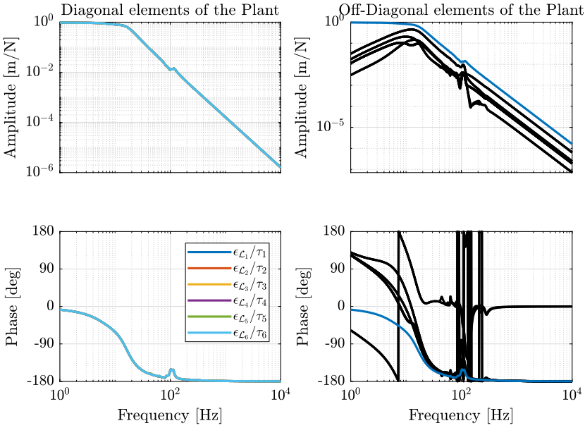
1.4.2 Obtained Plant

Figure 6: Obtained Primary plant in the Task space (png, pdf)

Figure 7: Obtained Primary plant in the frame of the legs (png, pdf)

1.4.3 Controller Design

wc = 2*pi*200; % Bandwidth Bandwidth [rad/s]

h = 2; % Lead parameter

Kp = (1/h) * (1 + s/wc*h)/(1 + s/wc/h) * ...
     (1/h) * (1 + s/wc*h)/(1 + s/wc/h); % For Piezo
% Kp = (1/h) * (1 + s/wc*h)/(1 + s/wc/h) * (s + 2*pi*10)/s * (s + 2*pi*1)/s ; % For voice coil

% Normalization of the gain of have a loop gain of 1 at frequency wc
Kp = Kp.*diag(1./diag(abs(freqresp(Gpx*Kp, wc))));

Figure 8: Obtained Loop gain for the primary controller in the Task space (png, pdf)

And now we include the Jacobian inside the controller.

Kp = inv(nano_hexapod.kinematics.J')*Kp;

1.5 Simulation

Let’s first save the 3 controllers for further analysis:

save('mat/hac_lac_cascade_vc_controllers.mat', 'Kiff', 'Kl', 'Kp')

load('mat/conf_simulink.mat');
set_param(conf_simulink, 'StopTime', '2');

And we simulate the system.

sim('nass_model');

cascade_hac_lac_lorentz = simout;
save('./mat/cascade_hac_lac.mat', 'cascade_hac_lac_lorentz', '-append');

1.6 Results

1.6.1 Load the simulation results

load('./mat/experiment_tomography.mat', 'tomo_align_dist');
load('./mat/cascade_hac_lac.mat', 'cascade_hac_lac', 'cascade_hac_lac_lorentz');

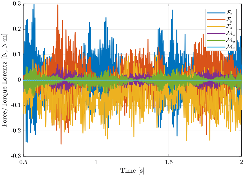
1.6.2 Control effort

Figure 9: Actuator Action during a tomography experiment when using Voice Coil actuators (png, pdf)

1.6.3 Load the simulation results

n_av = 4;
han_win = hanning(ceil(length(cascade_hac_lac.Em.En.Data(:,1))/n_av));

t = cascade_hac_lac.Em.En.Time;
Ts = t(2)-t(1);

[pxx_ol, f] = pwelch(tomo_align_dist.Em.En.Data, han_win, [], [], 1/Ts);
[pxx_ca, ~] = pwelch(cascade_hac_lac.Em.En.Data, han_win, [], [], 1/Ts);
[pxx_vc, ~] = pwelch(cascade_hac_lac_lorentz.Em.En.Data, han_win, [], [], 1/Ts);

Figure 10: Power Spectral Density of the position error during a tomography experiment when using Voice Coil based nano-hexapod (png, pdf)

Figure 11: Cumulative Amplitude Spectrum of the position error during a tomography experiment when using Voice Coil based nano-hexapod (png, pdf)

Figure 12: Position error during a tomography experiment when using Voice Coil based nano-hexapod (png, pdf)

1.7 Compliance of the nano-hexapod

1.7.1 Identification

Let’s identify the Compliance of the NASS:

%% Name of the Simulink File
mdl = 'nass_model';

%% Input/Output definition
clear io; io_i = 1;
io(io_i) = linio([mdl, '/Disturbances/Fd'], 1, 'openinput');       io_i = io_i + 1; % Direct Forces/Torques applied on the sample
io(io_i) = linio([mdl, '/Tracking Error'], 1, 'output', [], 'En'); io_i = io_i + 1; % Position Errror

First in open-loop:

Kp = tf(zeros(6));
Kl = tf(zeros(6));
Kiff = tf(zeros(6));

%% Run the linearization
Gc_ol = linearize(mdl, io, 0);
Gc_ol.InputName  = {'Fdx', 'Fdy', 'Fdz', 'Mdx', 'Mdy', 'Mdz'};
Gc_ol.OutputName = {'Ex', 'Ey', 'Ez', 'Erx', 'Ery', 'Erz'};

Then with the IFF control.

load('mat/hac_lac_cascade_vc_controllers.mat', 'Kiff')

%% Run the linearization
Gc_iff = linearize(mdl, io, 0);
Gc_iff.InputName  = {'Fdx', 'Fdy', 'Fdz', 'Mdx', 'Mdy', 'Mdz'};
Gc_iff.OutputName = {'Ex', 'Ey', 'Ez', 'Erx', 'Ery', 'Erz'};

With the HAC control added

load('mat/hac_lac_cascade_vc_controllers.mat', 'Kl')

%% Run the linearization
Gc_hac = linearize(mdl, io, 0);
Gc_hac.InputName  = {'Fdx', 'Fdy', 'Fdz', 'Mdx', 'Mdy', 'Mdz'};
Gc_hac.OutputName = {'Ex', 'Ey', 'Ez', 'Erx', 'Ery', 'Erz'};

Finally with the primary controller

load('mat/hac_lac_cascade_vc_controllers.mat', 'Kp')

%% Run the linearization
Gc_pri = linearize(mdl, io, 0);
Gc_pri.InputName  = {'Fdx', 'Fdy', 'Fdz', 'Mdx', 'Mdy', 'Mdz'};
Gc_pri.OutputName = {'Ex', 'Ey', 'Ez', 'Erx', 'Ery', 'Erz'};

1.7.2 Obtained Compliance

Figure 13: Evolution of the NASS compliance with each control loop added (png, pdf)

1.7.3 Comparison with Piezo

Let’s initialize a nano-hexapod with piezoelectric actuators.

initializeNanoHexapod('actuator', 'piezo');

We don’t use any controller.

Kp = tf(zeros(6));
Kl = tf(zeros(6));
Kiff = tf(zeros(6));

%% Run the linearization
Gc_pz = linearize(mdl, io, 0);
Gc_pz.InputName  = {'Fdx', 'Fdy', 'Fdz', 'Mdx', 'Mdy', 'Mdz'};
Gc_pz.OutputName = {'Ex', 'Ey', 'Ez', 'Erx', 'Ery', 'Erz'};

Figure 14: Comparison of the compliance using the open-loop piezo-nano hexapod and the voice coil nano-hexapod with the cascade control topology (png, pdf)

1.8 Robustness to Payload Variability

1.8.1 Initialization

Let’s change the payload mass, and see if the controller design for a payload mass of 1 still gives good performance.

initializeSample('mass', 50);

Kp = tf(zeros(6));
Kl = tf(zeros(6));
Kiff = tf(zeros(6));

1.8.2 Low Authority Control

Let’s first identify the transfer function for the Low Authority control.

%% Name of the Simulink File
mdl = 'nass_model';

%% Input/Output definition
clear io; io_i = 1;
io(io_i) = linio([mdl, '/Controller'],    1, 'openinput');               io_i = io_i + 1; % Actuator Inputs
io(io_i) = linio([mdl, '/Micro-Station'], 3, 'openoutput', [], 'Fnlm');  io_i = io_i + 1; % Force Sensors

%% Run the linearization
G_iff_m = linearize(mdl, io, 0);
G_iff_m.InputName  = {'Fnl1', 'Fnl2', 'Fnl3', 'Fnl4', 'Fnl5', 'Fnl6'};
G_iff_m.OutputName = {'Fnlm1', 'Fnlm2', 'Fnlm3', 'Fnlm4', 'Fnlm5', 'Fnlm6'};

The obtained dynamics is compared when using a payload of 1Kg in Figure 15.

Figure 15: Dynamics of the LAC plant when using a 50Kg payload (dashed) and when using a 1Kg payload (solid) (png, pdf)

A gain of 50 will here suffice to obtain critical damping of the nano-hexapod modes.

Let’s load the IFF controller designed when the payload has a mass of 1Kg.

load('mat/hac_lac_cascade_vc_controllers.mat', 'Kiff')

Figure 16: Loop gain for the IFF Control when using a 50Kg payload (dashed) and when using a 1Kg payload (solid) (png, pdf)

1.8.3 High Authority Control

We use the Integral Force Feedback developed with a mass of 1Kg and we identify the dynamics for the High Authority Controller in the case of the 50Kg payload

%% Name of the Simulink File
mdl = 'nass_model';

%% Input/Output definition
clear io; io_i = 1;
io(io_i) = linio([mdl, '/Controller'],    1, 'input');               io_i = io_i + 1; % Actuator Inputs
io(io_i) = linio([mdl, '/Micro-Station'], 3, 'output', [], 'Dnlm');  io_i = io_i + 1; % Leg Displacement

%% Run the linearization
Gl_m = linearize(mdl, io, 0);
Gl_m.InputName  = {'Fnl1', 'Fnl2', 'Fnl3', 'Fnl4', 'Fnl5', 'Fnl6'};
Gl_m.OutputName = {'Dnlm1', 'Dnlm2', 'Dnlm3', 'Dnlm4', 'Dnlm5', 'Dnlm6'};

isstable(Gl_m)
Gl_m = minreal(Gl_m);
isstable(Gl_m)

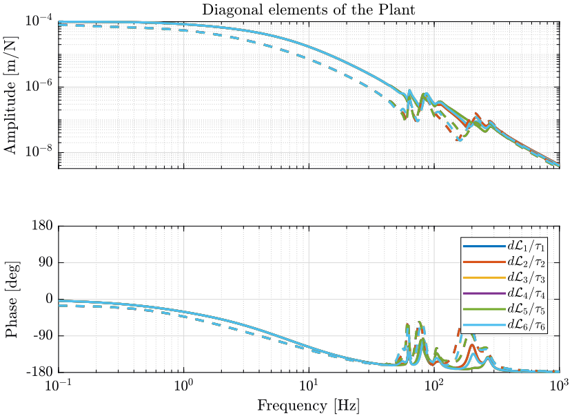
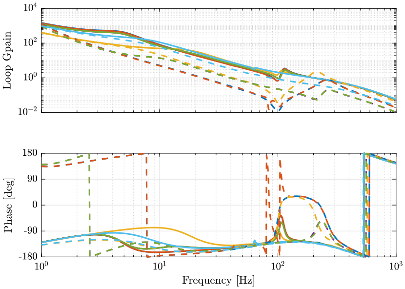
Figure 17: Dynamics of the HAC plant when using a 50Kg payload (dashed) and when using a 1Kg payload (solid) (png, pdf)

We load the HAC controller design when the payload has a mass of 1Kg.

load('mat/hac_lac_cascade_vc_controllers.mat', 'Kl')

Figure 18: Loop Gain of the HAC when using a 50Kg payload (dashed) and when using a 1Kg payload (solid) (png, pdf)

1.8.4 Primary Plant

We use the Low Authority Controller developed with a mass of 1Kg and we identify the dynamics for the Primary controller in the case of the 50Kg payload.

%% Name of the Simulink File
mdl = 'nass_model';

%% Input/Output definition
clear io; io_i = 1;
io(io_i) = linio([mdl, '/Controller/Cascade-HAC-LAC/Kp'],  1, 'input'); io_i = io_i + 1;
io(io_i) = linio([mdl, '/Tracking Error'], 1, 'output', [], 'En');      io_i = io_i + 1; % Position Errror

%% Run the linearization
Gp_m = linearize(mdl, io, 0);
Gp_m.InputName  = {'rl1', 'rl2', 'rl3', 'rl4', 'rl5', 'rl6'};
Gp_m.OutputName = {'Ex', 'Ey', 'Ez', 'Erx', 'Ery', 'Erz'};

A minus sign is added to cancel the minus sign already included in the identified plant.

isstable(Gp_m)
Gp_m = -minreal(Gp_m);
isstable(Gp_m)

load('mat/stages.mat', 'nano_hexapod');
Gpx_m = Gp_m*inv(nano_hexapod.kinematics.J');
Gpx_m.InputName  = {'Fx', 'Fy', 'Fz', 'Mx', 'My', 'Mz'};

Gpl_m = nano_hexapod.kinematics.J*Gp_m;
Gpl_m.OutputName  = {'El1', 'El2', 'El3', 'El4', 'El5', 'El6'};

There are two zeros with positive real part for the plant in the y direction at about 100Hz. This is problematic as it limits the bandwidth to be less than \(\approx 50\ \text{Hz}\).

It is important here to physically understand why such “positive” zero appears.

If we make a “rigid” 50kg paylaod, the positive zero disappears.

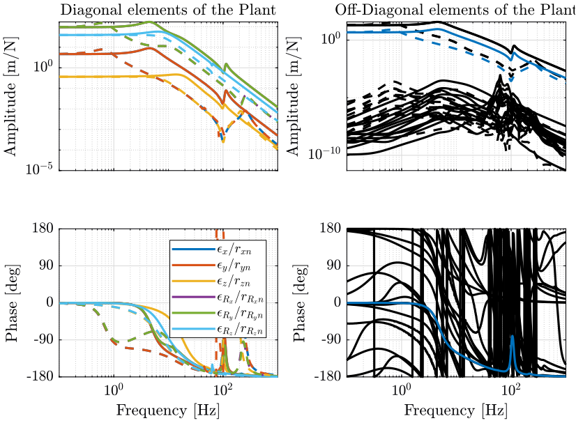
Figure 19: Dynamics of the Primary plant when using a 50Kg payload (dashed) and when using a 1Kg payload (solid) (png, pdf)

We load the primary controller that was design when the payload has a mass of 1Kg.

We load the HAC controller design when the payload has a mass of 1Kg.

load('mat/hac_lac_cascade_vc_controllers.mat', 'Kp')
Kp_x = nano_hexapod.kinematics.J'*Kp;

wc = 2*pi*50; % Bandwidth Bandwidth [rad/s]

h = 2; % Lead parameter

Kp = (1/h) * (1 + s/wc*h)/(1 + s/wc/h) * ...
     (1/h) * (1 + s/wc*h)/(1 + s/wc/h) * ...
     (s + 2*pi*1)/s * ...
     1/(1+s/2/wc); % For Piezo

% Normalization of the gain of have a loop gain of 1 at frequency wc
Kp = Kp.*diag(1./diag(abs(freqresp(Gpx_m*Kp, wc))));

Figure 20: Loop Gain of the Primary loop when using a 50Kg payload (dashed) and when using a 1Kg payload (solid) (png, pdf)

1.8.5 Simulation

load('mat/conf_simulink.mat');
set_param(conf_simulink, 'StopTime', '2');

And we simulate the system.

sim('nass_model');

cascade_hac_lac_lorentz_high_mass = simout;
save('./mat/cascade_hac_lac.mat', 'cascade_hac_lac_lorentz_high_mass', '-append');

load('./mat/experiment_tomography.mat', 'tomo_align_dist');

2 Other analysis

2.1 Robustness to Payload Variability

[ ] For 3/masses (1kg, 10kg, 50kg), plot each of the 3 plants

2.2 Direct HAC control in the task space - \(\bm{K}_\mathcal{X}\)

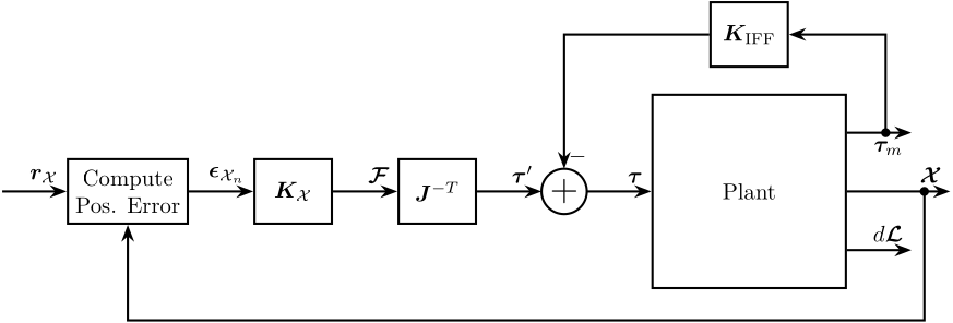
Figure 21: Control Architecture containing an IFF controller and a Controller in the task space

2.2.1 Identification

initializeController('type', 'hac-iff');

%% Name of the Simulink File
mdl = 'nass_model';

%% Input/Output definition
clear io; io_i = 1;
io(io_i) = linio([mdl, '/Controller/HAC-IFF/Kx'],  1, 'input');    io_i = io_i + 1; % Control input
io(io_i) = linio([mdl, '/Tracking Error'], 1, 'output', [], 'En'); io_i = io_i + 1; % Position Errror

%% Run the linearization
G = linearize(mdl, io, 0);
G.InputName  = {'Fnl1', 'Fnl2', 'Fnl3', 'Fnl4', 'Fnl5', 'Fnl6'};
G.OutputName = {'Ex', 'Ey', 'Ez', 'Erx', 'Ery', 'Erz'};

isstable(G)
G = -minreal(G);
isstable(G)

load('mat/stages.mat', 'nano_hexapod');
Gx = G*inv(nano_hexapod.kinematics.J');
Gx.InputName  = {'Fx', 'Fy', 'Fz', 'Mx', 'My', 'Mz'};

Gl = nano_hexapod.kinematics.J*G;
Gl.OutputName  = {'El1', 'El2', 'El3', 'El4', 'El5', 'El6'};

2.2.2 Obtained Plant in the Task Space

2.2.3 Obtained Plant in the Joint Space

2.2.4 Controller Design in the Joint Space

wc = 2*pi*200; % Bandwidth Bandwidth [rad/s]

h = 2; % Lead parameter

Kx = (1/h) * (1 + s/wc*h)/(1 + s/wc/h) * ... % Lead
     (1/h) * (1 + s/wc*h)/(1 + s/wc/h) * ... % Lead
     (s + 2*pi*10)/s * ... % Pseudo Integrator
     1/(1+s/2/pi/500); % Low pass Filter

% Normalization of the gain of have a loop gain of 1 at frequency wc
Kx = Kx.*diag(1./diag(abs(freqresp(Gx*Kx, wc))));

wc = 2*pi*200; % Bandwidth Bandwidth [rad/s]

h = 2; % Lead parameter

Kl = (1/h) * (1 + s/wc*h)/(1 + s/wc/h) * ... % Lead
     (1/h) * (1 + s/wc*h)/(1 + s/wc/h) * ... % Lead
     (s + 2*pi*1)/s * ... % Pseudo Integrator
     (s + 2*pi*10)/s * ... % Pseudo Integrator
     1/(1+s/2/pi/500); % Low pass Filter

% Normalization of the gain of have a loop gain of 1 at frequency wc
Kl = Kl.*diag(1./diag(abs(freqresp(Gl*Kl, wc))));

2.3 On the usefulness of the High Authority Control loop / Linearization loop

Let’s see what happens is we omit the HAC loop and we directly try to control the damped plant using the measurement of the sample with respect to the granite \(\bm{\mathcal{X}}\).

We can do that in two different ways:

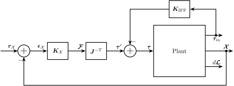
in the task space as shown in Figure 22
in the space of the legs as shown in Figure 23

Figure 22: IFF control + primary controller in the task space

Figure 23: HAC-LAC control architecture in the frame of the legs

2.3.1 Identification

initializeController('type', 'hac-iff');

%% Name of the Simulink File
mdl = 'nass_model';

%% Input/Output definition
clear io; io_i = 1;
io(io_i) = linio([mdl, '/Controller/HAC-IFF/Kx'],  1, 'input');    io_i = io_i + 1;
io(io_i) = linio([mdl, '/Tracking Error'], 1, 'output', [], 'En'); io_i = io_i + 1; % Position Errror

%% Run the linearization
G = linearize(mdl, io, 0);
G.InputName  = {'F1', 'F2', 'F3', 'F4', 'F5', 'F6'};
G.OutputName = {'Ex', 'Ey', 'Ez', 'Erx', 'Ery', 'Erz'};

isstable(G)
G = -minreal(G);
isstable(G)

2.3.2 Plant in the Task space

The obtained plant is shown in Figure

Gx = G*inv(nano_hexapod.kinematics.J');

2.3.3 Plant in the Leg’s space

Gl = nano_hexapod.kinematics.J*G;

2.4 DVF instead of IFF?

2.4.1 Initialization and Identification

initializeController('type', 'hac-dvf');
Kdvf = tf(zeros(6));

%% Name of the Simulink File
mdl = 'nass_model';

%% Input/Output definition
clear io; io_i = 1;
io(io_i) = linio([mdl, '/Controller'],    1, 'openinput');               io_i = io_i + 1; % Actuator Inputs
io(io_i) = linio([mdl, '/Micro-Station'], 3, 'openoutput', [], 'Dnlm');  io_i = io_i + 1; % Displacement Sensors

%% Run the linearization
G_dvf = linearize(mdl, io, 0);
G_dvf.InputName  = {'Fnl1', 'Fnl2', 'Fnl3', 'Fnl4', 'Fnl5', 'Fnl6'};
G_dvf.OutputName = {'Dlm1', 'Dlm2', 'Dlm3', 'Dlm4', 'Dlm5', 'Dlm6'};

2.4.2 Obtained Plant

2.4.3 Controller

Kdvf = -850*s/(1+s/2/pi/1000)*eye(6);

2.4.4 HAC Identification

%% Name of the Simulink File
mdl = 'nass_model';

%% Input/Output definition
clear io; io_i = 1;
io(io_i) = linio([mdl, '/Controller/HAC-DVF/Kx'],  1, 'input');    io_i = io_i + 1; % Control input
io(io_i) = linio([mdl, '/Tracking Error'], 1, 'output', [], 'En'); io_i = io_i + 1; % Position Errror

%% Run the linearization
G = linearize(mdl, io, 0);
G.InputName  = {'Fnl1', 'Fnl2', 'Fnl3', 'Fnl4', 'Fnl5', 'Fnl6'};
G.OutputName = {'Ex', 'Ey', 'Ez', 'Erx', 'Ery', 'Erz'};

isstable(G)
G = -minreal(G);
isstable(G)

load('mat/stages.mat', 'nano_hexapod');
Gx = G*inv(nano_hexapod.kinematics.J');
Gx.InputName  = {'Fx', 'Fy', 'Fz', 'Mx', 'My', 'Mz'};

Gl = nano_hexapod.kinematics.J*G;
Gl.OutputName  = {'El1', 'El2', 'El3', 'El4', 'El5', 'El6'};

2.4.5 Conclusion

DVF can be used instead of IFF.