Effect of Uncertainty on the payload’s dynamics on the isolation platform dynamics
Table of Contents
- 1. Simple Introductory Example
- 2. Generalization to arbitrary dynamics
- 2.1. Introduction
- 2.2. Equations of motion
- 2.3. Impedance \(G^\prime(s)\) of a mass-spring-damper payload
- 2.4. First Analytical analysis
- 2.5. Impedance of the Payload and Dynamical Uncertainty
- 2.6. Equivalent Inverse Multiplicative Uncertainty
- 2.7. Effect of the Isolation platform Stiffness
- 2.8. Reduce the Uncertainty on the plant
- 2.9. Conclusion
In this document we will consider an isolation platform (e.g. the nano-hexapod) with a payload on top (e.g. the the sample to be positioned).
The goal is to study:
- how does the dynamics of the payload influence the dynamics of the isolation platform
- similarly: how does the uncertainty on the payload’s dynamics will be transferred to uncertainty on the plant
- what design choice should be made in order to minimize the resulting uncertainty on the plant
Two models are made to study these effects:
- In section 1, simple mass-spring-damper systems are chosen to model both the isolation platform and the payload
- In section 2, we consider arbitrary payload dynamics with multiplicative input uncertainty to study the unmodelled dynamics of the payload
1 Simple Introductory Example
Let’s consider the system shown in Figure 1 consisting of:
- An isolation platform represented by a mass \(m\), a stiffness \(k\) and a dashpot \(c\) and an actuator \(F\)
- A payload represented by a mass \(m^\prime\), a stiffness \(k^\prime\) and a dashpot \(c^\prime\)
The goal is to stabilize \(x\) using \(F\) in spite of uncertainty on the payload mechanical properties.
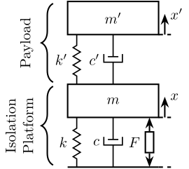
Figure 1: Two degrees-of-freedom system
1.1 Equations of motion
If we write the equation of motion of the system in Figure 1, we obtain:
\begin{align} ms^2 x &= F - (cs + k) x + (c^\prime s + k^\prime) (x^\prime - x) \\ m^\prime s^2 x^\prime &= - (c^\prime s + k^\prime) (x^\prime - x) \end{align}After eliminating \(x^\prime\), we obtain:
\begin{equation} \label{orge5d69a3} \frac{x}{F} = \frac{m^\prime s^2 + c^\prime s + k^\prime}{(ms^2 + cs + k)(m^\prime s^2 + c^\prime s + k^\prime) + m^\prime s^2(c^\prime s + k^\prime)} \end{equation}1.2 Initialization of the payload dynamics
Let the payload have:
- a nominal mass of \(m^\prime = 50\ [kg]\)
- a nominal stiffness of \(k^\prime = 5 \cdot 10^6\ [N/m]\)
- a nominal damping of \(c^\prime = 3 \cdot 10^3\ [N/(m/s)]\)
mpi = 50;
kpi = 5e6;
cpi = 3e3;

kpi = (2*pi*50)^2*mpi;
cpi = 0.2*sqrt(kpi*mpi);
Let’s also consider some uncertainty in those parameters:
mp = ureal('m', mpi, 'Range', [1, 100]);
cp = ureal('c', cpi, 'Percentage', 30);
kp = ureal('k', kpi, 'Percentage', 30);
The compliance of the payload without the isolation platform is \(\frac{1}{m^\prime s^2 + c^\prime s + k^\prime}\) and its bode plot is shown in Figure 2.
One can see that the payload has a resonance frequency of \(\omega_0^\prime = 250\ Hz\).
1.3 Initialization of the isolation platform
Let’s first fix the mass of the isolation platform:
m = 10;
And we generate three isolation platforms:
- A soft one with \(\omega_0 = 0.1 \omega_0^\prime = 5\ Hz\)
- A medium stiff one with \(\omega_0 = \omega_0^\prime = 50\ Hz\)
- A stiff one with \(\omega_0 = 10 \omega_0^\prime = 500\ Hz\)
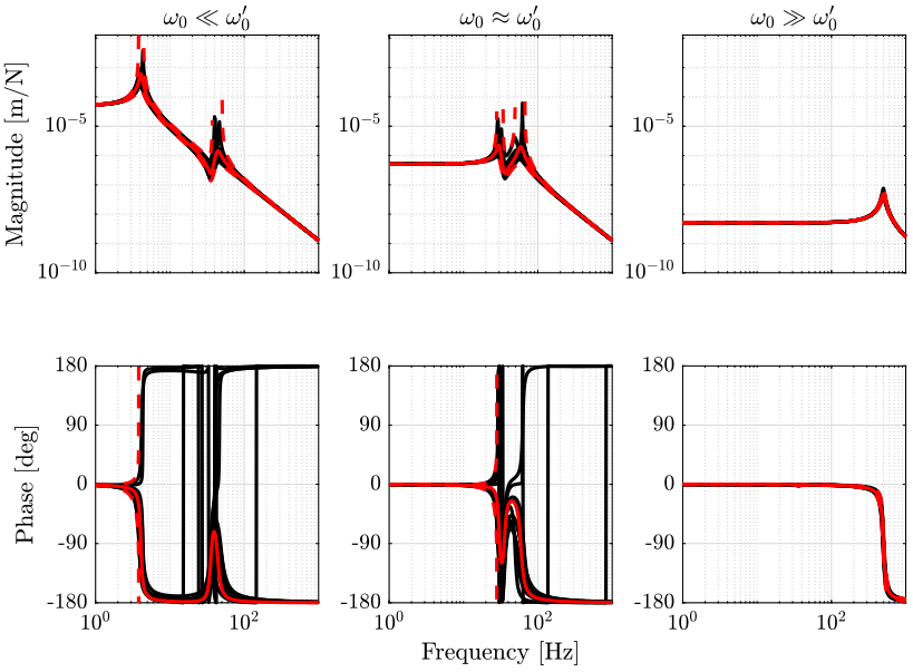
1.4 Comparison
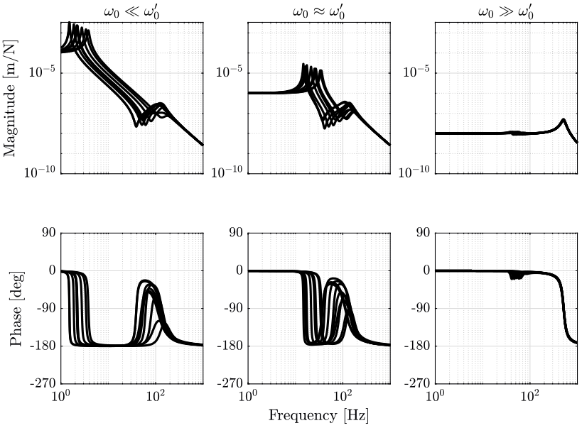
1.5 Conclusion
The stiff platform dynamics does not seems to depend on the dynamics of the payload.
2 Generalization to arbitrary dynamics
2.1 Introduction
Let’s now consider a general payload described by its impedance \(G^\prime(s) = \frac{F^\prime}{x}\) as shown in Figure 4.
Note here that we use the term impedance, however, the mechanical impedance is usually defined as the ratio of the force over the velocity \(F^\prime/\dot{x}\). We should refer to resistance instead of impedance.

Figure 4: General support
Now let’s consider the system consisting of a mass-spring-system (the isolation platform) supporting the general payload as shown in Figure 5.
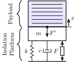
Figure 5: Mass-Spring-Damper (isolation platform) supporting a general payload
2.2 Equations of motion
We have to following equations of motion:
\begin{align} ms^2 x &= F - (cs + k) x - F^\prime \\ F^\prime &= G^\prime(s) x \end{align}And by eliminating \(F^\prime\), we find the plant dynamics \(G(s) = \frac{x}{F}\).
We can learn few things about the obtained transfer function:
- the zeros of \(x/F\) will be the poles of \(G^\prime(s)\).
- if the impedance of the payload is small \(|G^\prime(s)| \ll |ms^2 + cs + k|\), then the payload will have small influence on the obtained dynamics
2.3 Impedance \(G^\prime(s)\) of a mass-spring-damper payload
In order to verify that the formula is correct, let’s take the same mass-spring-damper system used in the system shown in Figure 1:
\begin{align*} m^\prime s^2 x^\prime &= (x - x^\prime) (c^\prime s + k^\prime) \\ F^\prime &= (x - x^\prime) (c^\prime s + k^\prime) \end{align*}By eliminating \(x^\prime\) of the equations, we obtain:
The impedance of a 1dof mass-spring-damper system is described by Eq. \eqref{eq:impedance_mass_spring_damper}.
And we obtain
\begin{align*} \frac{x}{F} &= \frac{1}{ms^2 + cs + k + G^\prime(s)} \\ &= \frac{1}{ms^2 + cs + k + \frac{m^\prime s^2 (c^\prime s + k)}{m^\prime s^2 + c^\prime s + k^\prime}} \\ &= \frac{m^\prime s^2 + c^\prime s + k^\prime}{(ms^2 + cs + k) (m^\prime s^2 + c^\prime s + k^\prime) + m^\prime s^2 (c^\prime s + k)} \end{align*}Which is the same transfer function that was obtained in section 1 (Eq. \eqref{eq:plant_simple_system}).
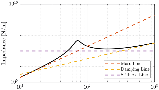
The impedance of the mass-spring-damper system is shown in Figure 6.
- Before the resonance frequency \(\omega_0^\prime\), the impedance follows the mass line
- After the resonance, the impedance will follow the stiffness line (depending on the relative values of the stiffness and damping)
- At high frequency, it will follow the damping line
2.4 First Analytical analysis
To summarize, we consider:
- an Isolation platform represented by a mass \(m\), a damper \(c\) and a stiffness \(k\). This system resonate at \(\omega_0 = \sqrt{\frac{k}{m}}\)
- A payload represented by a mass \(m^\prime\), a damper \(c^\prime\) and a stiffness \(k^\prime\). The payload resonate at \(\omega_0^\prime = \sqrt{\frac{k^\prime}{m^\prime}}\)
The “impedance” of the payload is represented by: \[ G^\prime(s) = \frac{m^\prime s^2 (c^\prime s + k^\prime)}{m^\prime s^2 + c^\prime s + k^\prime} \]
And the plant is: \[ G(s) = \frac{x}{F} = \frac{1}{ms^2 + cs + k + G^\prime(s)} \]
Let’s write the asymptotic behavior of \(|G^\prime(j\omega)|\):
- \(\lim_{\omega \to 0} |G^\prime(j\omega)| = m^\prime s^2\)
- \(|G^\prime(j\omega_0)| = \frac{k^\prime \sqrt{1 + (2\xi^\prime)^2}}{2 \xi^\prime}\)
- \(\lim_{\omega \to \infty} |G^\prime(j\omega)| = c^\prime s + k\)
Let’s find some conditions in order to have that the dynamics of the payload does not influence to much the dynamics of the plant: \[ |G^\prime(s)| \ll |ms^2 + cs + k| \]
Let’s take the case of a stiff payload (\(\omega_0^\prime \gg \omega_0\)).
Below \(\omega_0\), the condition becomes: \[ |G^\prime(s)| \ll k \Leftrightarrow m^\prime \omega_0^2 \ll k \Leftrightarrow m^\prime \ll m \] The payload mass should be small with respect to the isolation platform mass.
Above \(\omega_0\): \[ |G^\prime(j\omega)| \ll m \omega^2 \]
Until \(\omega_0^\prime\), we have \(m^\prime \ll m\) which is the same condition as before. Above \(\omega_0^\prime\), we obtain \(|jc^\prime \omega + k| \ll m \omega^2\).
When using a soft isolation platform and a stiff payload such that the payload resonate above the first resonance of the isolation platform, the mass of the payload should be small compared to the isolation platform mass in order to not disturb the dynamics of the isolation platform.
2.5 Impedance of the Payload and Dynamical Uncertainty
We model the payload by a mass-spring-damper model with some uncertainty.
Let the payload have:
- a nominal mass of \(m^\prime = 50\ [kg]\)
- a nominal stiffness of \(k^\prime = 5 \cdot 10^6\ [N/m]\)
- a nominal damping of \(c^\prime = 3 \cdot 10^3\ [N/(m/s)]\)
The main resonance of the payload is then \(\omega^\prime = \sqrt{\frac{m^\prime}{k^\prime}} \approx 50\ Hz\).
m0 = 10;
c0 = 3e2;
k0 = 5e5;

Gp0 = (m0*s^2 * (c0*s + k0))/(m0*s^2 + c0*s + k0);
Let’s represent the uncertainty on the impedance of the payload by a multiplicative uncertainty (Figure 7): \[ G^\prime(s) = G_0^\prime(s)(1 + w_I^\prime(s)\Delta_I(s)) \quad |\Delta_I(j\omega)| < 1\ \forall \omega \]
This could represent unmodelled dynamics or unknown parameters of the payload.
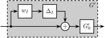
Figure 7: Input Multiplicative Uncertainty
We choose a simple uncertainty weight: \[ w_I(s) = \frac{\tau s + r_0}{(\tau/r_\infty) s + 1} \] where \(r_0\) is the relative uncertainty at steady-state, \(1/\tau\) is the frequency at which the relative uncertainty reaches \(100\ \%\), and \(r_\infty\) is the magnitude of the weight at high frequency.
The parameters are defined below.
r0 = 0.5;
tau = 1/(50*2*pi);
rinf = 10;

wI = (tau*s + r0)/((tau/rinf)*s + 1);
We then generate a complex \(\Delta\).
DeltaI = ucomplex('A',0);
We generate the uncertain plant \(G^\prime(s)\).
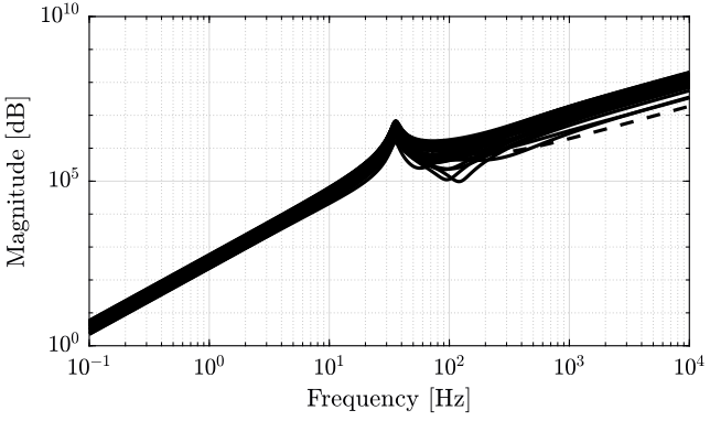
Gp = Gp0*(1+wI*DeltaI);
A set of uncertainty payload’s impedance transfer functions is shown in Figure 8.
2.6 Equivalent Inverse Multiplicative Uncertainty
Let’s express the uncertainty of the plant \(x/F\) as a function of the parameters as well as of the uncertainty on the platform’s compliance:
\begin{align*} \frac{x}{F} &= \frac{1}{ms^2 + cs + k + G_0^\prime(s)(1 + w_I(s)\Delta(s))}\\ &= \frac{1}{ms^2 + cs + k + G_0^\prime(s)} \cdot \frac{1}{1 + \frac{G_0^\prime(s) w_I(s)}{ms^2 + cs + k + G_0^\prime(s)} \Delta(s)}\\ \end{align*}We can the plant dynamics that as an inverse multiplicative uncertainty (Figure 9):
\begin{equation} \frac{x}{F} = G_0(s) (1 + w_{iI}(s) \Delta(s))^{-1} \end{equation}with:
- \(G_0(s) = \frac{1}{ms^2 + cs + k + G_0^\prime(s)}\)
- \(w_{iI}(s) = \frac{G_0^\prime(s) w_I(s)}{ms^2 + cs + k + G_0^\prime(s)} = G_0(s) G_0^\prime(s) w_I(s)\)
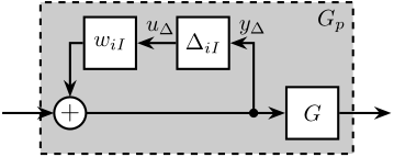
Figure 9: Inverse Multiplicative Uncertainty
2.7 Effect of the Isolation platform Stiffness
Let’s first fix the mass of the isolation platform:
m = 20;
And we generate three isolation platforms:
- A soft one with \(\omega_0 = 5\ Hz\)
- A medium stiff one with \(\omega_0 = 50\ Hz\)
- A stiff one with \(\omega_0 = 500\ Hz\)
Soft Isolation Platform:
k_soft = m*(2*pi*5)^2;
c_soft = 0.1*sqrt(m*k_soft);

G_soft = 1/(m*s^2 + c_soft*s + k_soft + Gp);
G0_soft = 1/(m*s^2 + c_soft*s + k_soft + Gp0);
wiI_soft = Gp0*G0_soft*wI;
Mid Isolation Platform
k_mid = m*(2*pi*50)^2;
c_mid = 0.1*sqrt(m*k_mid);

G_mid = 1/(m*s^2 + c_mid*s + k_mid + Gp);
G0_mid = 1/(m*s^2 + c_mid*s + k_mid + Gp0);
wiI_mid = Gp0*G0_mid*wI;
Stiff Isolation Platform
k_stiff = m*(2*pi*500)^2;
c_stiff = 0.1*sqrt(m*k_stiff);

G_stiff = 1/(m*s^2 + c_stiff*s + k_stiff + Gp);
G0_stiff = 1/(m*s^2 + c_stiff*s + k_stiff + Gp0);
wiI_stiff = Gp0*G0_stiff*wI;
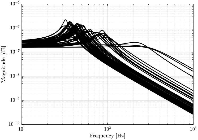
The obtained transfer functions \(x/F\) for each of the three platforms are shown in Figure 10.
2.8 Reduce the Uncertainty on the plant
Now that we know the expression of the uncertainty on the plant, we can wonder what parameters of the isolation platform would lower the plant uncertainty, or at least bring the uncertainty to reasonable level.
The uncertainty of the plant is described by an inverse multiplicative uncertainty with the following weight: \[ w_{iI}(s) = \frac{G_0^\prime(s) w_I(s)}{ms^2 + cs + k + G_0^\prime(s)} \]
Let’s study separately the effect of the platform’s mass, damping and stiffness.
2.8.1 Effect of the platform’s stiffness \(k\)
Let’s fix \(\xi = \frac{c}{2\sqrt{km}} = 0.1\), \(m = 100\ [kg]\) and see the evolution of \(|w_{iI}(j\omega)|\) with \(k\).
This is first shown for few values of the stiffness \(k\) in figure 11
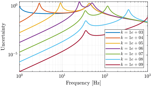
Figure 11: Norm of the inverse multiplicative uncertainty weight for various values of the the isolation platform’s stiffness (png, pdf)
The norm of the uncertainty weight \(|w_iI(j\omega)|\) is displayed as a function of \(\omega\) and \(k\) in Figure 12.
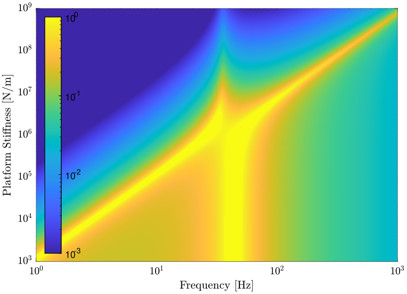
Figure 12: Evolution of the norm of the uncertainty weight \(|w_{iI}(j\omega)|\) as a function of the platform’s stiffness \(k\) (png, pdf)
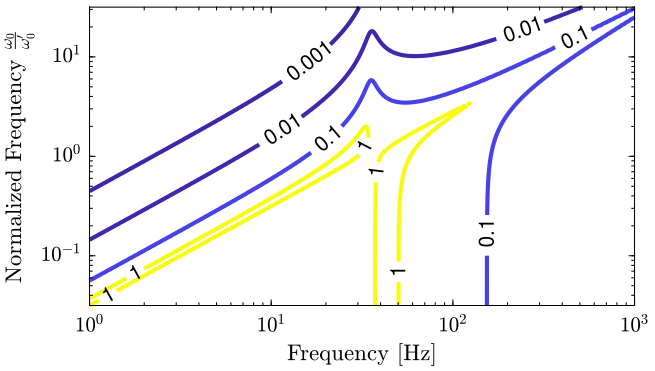
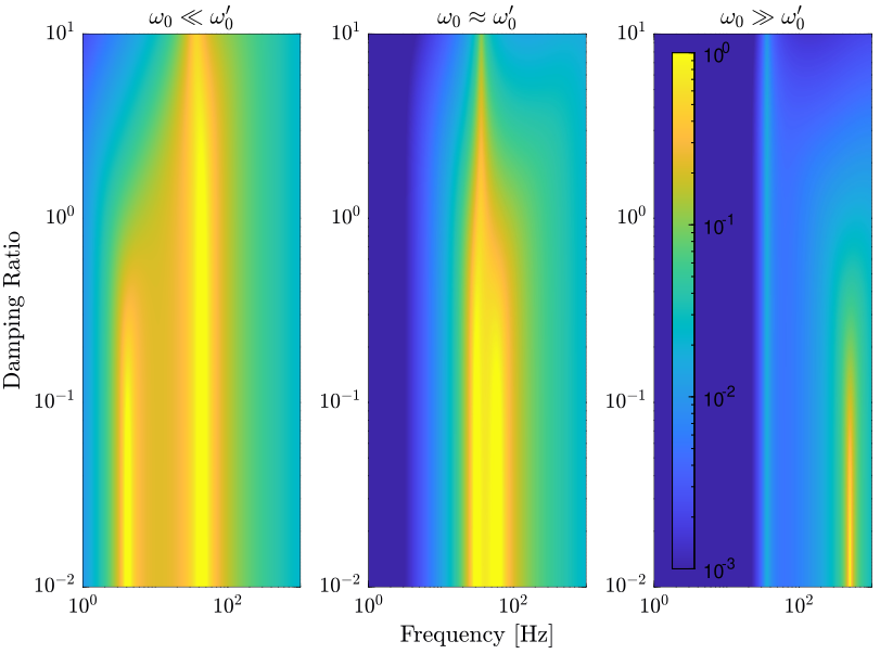
Instead of plotting as a function of the platform’s stiffness, we can plot as a function of \(\omega_0/\omega_0^\prime\) where:
- \(\omega_0\) is the resonance of the platform alone
- \(\omega_0^\prime\) is the resonance of the support alone
The obtain plot is shown in Figure 13. In that case, we can see that with a platform’s resonance frequency 10 times higher than the resonance of the payload, we get less than \(1\%\) uncertainty until some fairly high frequency.
2.8.2 Effect of the platform’s damping \(c\)
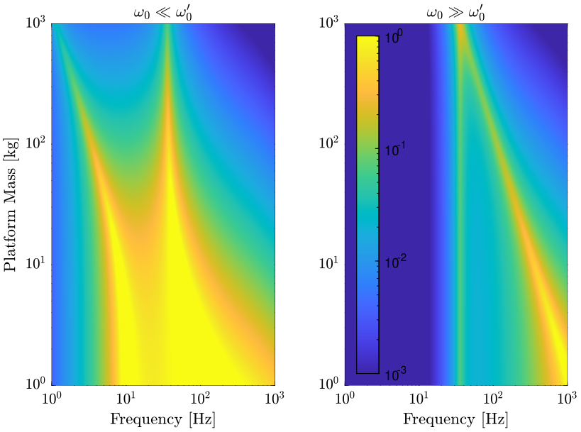
2.8.3 Effect of the platform’s mass \(m\)
2.9 Conclusion
As was expected from Eq. \eqref{org8b9a6a7}, it is usually a good idea to maximize the mass, damping and stiffness of the isolation platform in order to be less sensible to the payload dynamics.
The best thing to do is to have a stiff isolation platform.
If a soft isolation platform is to be used, it is first a good idea to damp the isolation platform as shown in Figure 14. This can make the uncertainty quite low until the first resonance of the payload. In that case, maximizing the stiffness of the payload is a good idea.