Active Damping with an uni-axial model
Table of Contents
First, in section 1, we will looked at the undamped system.
Then, we will compare three active damping techniques:
- In section 2: the integral force feedback is used
- In section 3: the relative motion control is used
- In section 4: the direct velocity feedback is used
For each of the active damping technique, we will:
- Compare the sensitivity from disturbances
- Look at the damped plant
The disturbances are:
- Ground motion
- Direct forces
- Motion errors of all the stages
1 Undamped System
All the files (data and Matlab scripts) are accessible here.
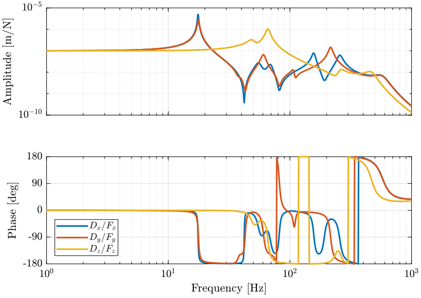
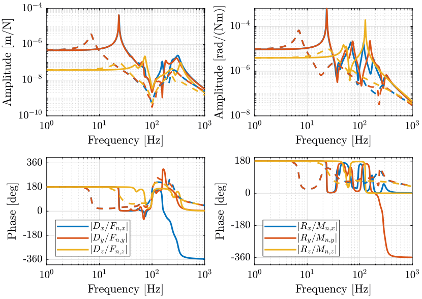
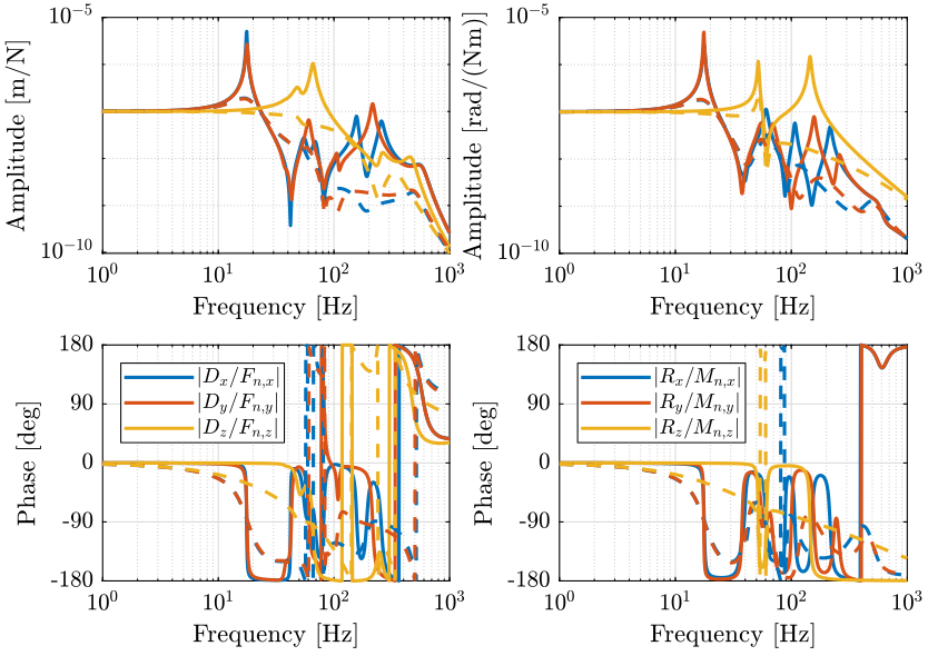
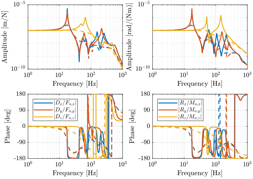
We first look at the undamped system. The performance of this undamped system will be compared with the damped system using various techniques.
1.1 Init
We initialize all the stages with the default parameters. The nano-hexapod is a piezoelectric hexapod and the sample has a mass of 50kg.
  initializeReferences();
  initializeGround();
  initializeGranite();
  initializeTy();
  initializeRy();
  initializeRz();
  initializeMicroHexapod();
  initializeAxisc();
  initializeMirror();
  initializeNanoHexapod('actuator', 'piezo');
  initializeSample('mass', 50);
All the controllers are set to 0.
  K = tf(zeros(6));
  save('./mat/controllers_uniaxial.mat', 'K', '-append');
  K_iff = tf(zeros(6));
  save('./mat/controllers_uniaxial.mat', 'K_iff', '-append');
  K_rmc = tf(zeros(6));
  save('./mat/controllers_uniaxial.mat', 'K_rmc', '-append');
  K_dvf = tf(zeros(6));
  save('./mat/controllers_uniaxial.mat', 'K_dvf', '-append');
1.2 Identification
We identify the various transfer functions of the system
G = identifyPlant();
And we save it for further analysis.
save('./mat/active_damping_uniaxial_plants.mat', 'G', '-append');
1.3 Sensitivity to disturbances
2 Integral Force Feedback
All the files (data and Matlab scripts) are accessible here.
Integral Force Feedback is applied. In section 2.1, IFF is applied on a uni-axial system to understand its behavior. Then, it is applied on the simscape model.
2.1 One degree-of-freedom example
2.1.1 Equations
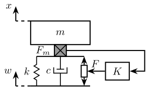
Figure 4: Integral Force Feedback applied to a 1dof system
The dynamic of the system is described by the following equation:
\begin{equation} ms^2x = F_d - kx - csx + kw + csw + F \end{equation}The measured force \(F_m\) is:
\begin{align} F_m &= F - kx - csx + kw + csw \\ &= ms^2 x - F_d \end{align}The Integral Force Feedback controller is \(K = -\frac{g}{s}\), and thus the applied force by this controller is:
\begin{equation} F_{\text{IFF}} = -\frac{g}{s} F_m = -\frac{g}{s} (ms^2 x - F_d) \end{equation}Once the IFF is applied, the new dynamics of the system is:
\begin{equation} ms^2x = F_d + F - kx - csx + kw + csw - \frac{g}{s} (ms^2x - F_d) \end{equation}And finally:
\begin{equation} x = F_d \frac{1 + \frac{g}{s}}{ms^2 + (mg + c)s + k} + F \frac{1}{ms^2 + (mg + c)s + k} + w \frac{k + cs}{ms^2 + (mg + c)s + k} \end{equation}We can see that this:
- adds damping to the system by a value \(mg\)
- lower the compliance as low frequency by a factor: \(1 + g/s\)
If we want critical damping:
\begin{equation} \xi = \frac{1}{2} \frac{c + gm}{\sqrt{km}} = \frac{1}{2} \end{equation}This is attainable if we have:
\begin{equation} g = \frac{\sqrt{km} - c}{m} \end{equation}2.1.2 Matlab Example
Let define the system parameters.
  m = 50; % [kg]
  k = 1e6; % [N/m]
  c = 1e3; % [N/(m/s)]
The state space model of the system is defined below.
  A = [-c/m -k/m;
       1     0];

  B = [1/m 1/m -1;
       0   0    0];

  C = [ 0  1;
       -c -k];

  D = [0 0 0;
       1 0 0];

  sys = ss(A, B, C, D);
  sys.InputName = {'F', 'Fd', 'wddot'};
  sys.OutputName = {'d', 'Fm'};
  sys.StateName = {'ddot', 'd'};
The controller \(K_\text{IFF}\) is:
  Kiff = -((sqrt(k*m)-c)/m)/s;
  Kiff.InputName = {'Fm'};
  Kiff.OutputName = {'F'};
And the closed loop system is computed below.
sys_iff = feedback(sys, Kiff, 'name', +1);
2.2 Control Design
Let’s load the undamped plant:
load('./mat/active_damping_uniaxial_plants.mat', 'G');
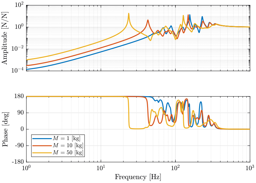
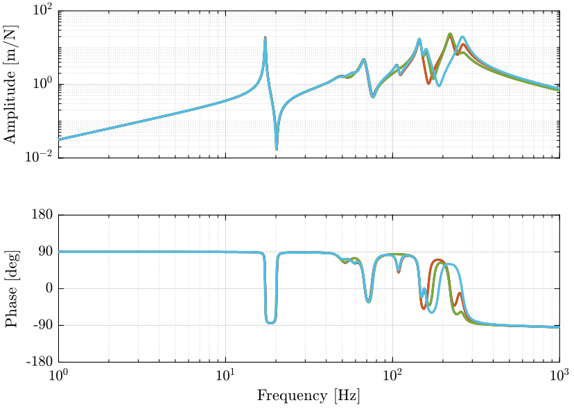
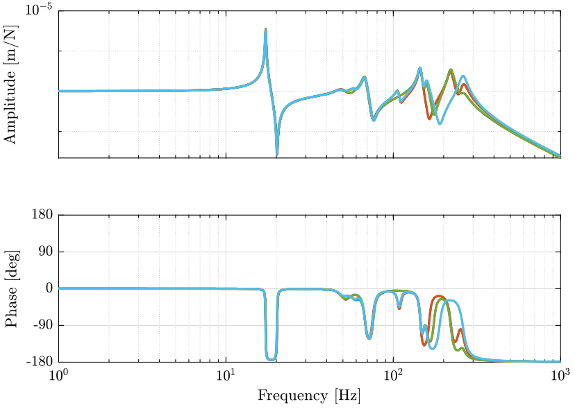
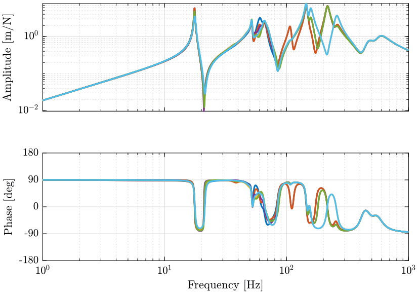
Let’s look at the transfer function from actuator forces in the nano-hexapod to the force sensor in the nano-hexapod legs for all 6 pairs of actuator/sensor (figure 6).
The controller for each pair of actuator/sensor is:
K_iff = -1000/s;
The corresponding loop gains are shown in figure 7.
2.3 Identification of the damped plant
Let’s initialize the system prior to identification.
  initializeReferences();
  initializeGround();
  initializeGranite();
  initializeTy();
  initializeRy();
  initializeRz();
  initializeMicroHexapod();
  initializeAxisc();
  initializeMirror();
  initializeNanoHexapod('actuator', 'piezo');
  initializeSample('mass', 50);
All the controllers are set to 0.
  K = tf(zeros(6));
  save('./mat/controllers_uniaxial.mat', 'K', '-append');
  K_iff = -K_iff*eye(6);
  save('./mat/controllers_uniaxial.mat', 'K_iff', '-append');
  K_rmc = tf(zeros(6));
  save('./mat/controllers_uniaxial.mat', 'K_rmc', '-append');
  K_dvf = tf(zeros(6));
  save('./mat/controllers_uniaxial.mat', 'K_dvf', '-append');
We identify the system dynamics now that the IFF controller is ON.
G_iff = identifyPlant();
And we save the damped plant for further analysis
save('./mat/active_damping_uniaxial_plants.mat', 'G_iff', '-append');
2.4 Sensitivity to disturbances
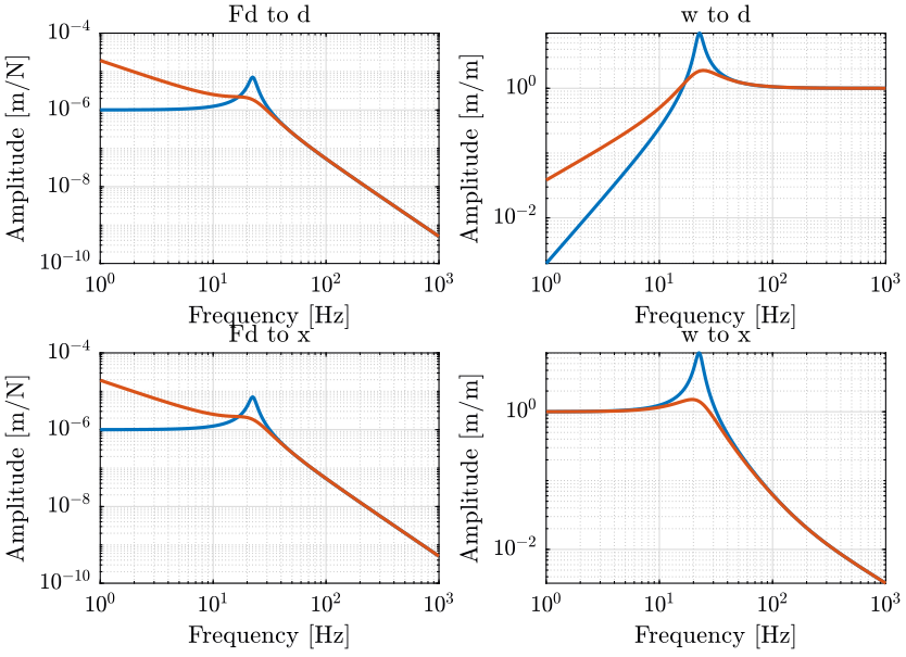
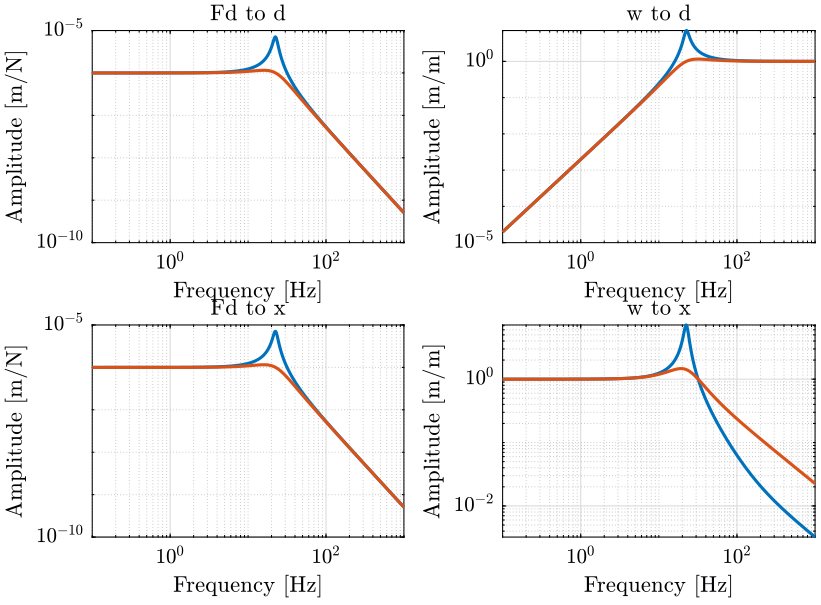
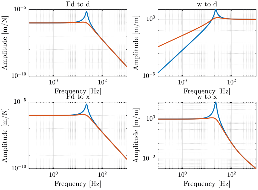
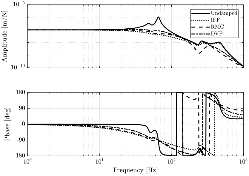
As shown on figure 8:
- The top platform of the nano-hexapod how behaves as a “free-mass”.
- The transfer function from direct forces \(F_s\) to the relative displacement \(D\) is equivalent to the one of an isolated mass.
- The transfer function from ground motion \(D_g\) to the relative displacement \(D\) tends to the transfer function from \(D_g\) to the displacement of the granite (the sample is being isolated thanks to IFF). However, as the goal is to make the relative displacement \(D\) as small as possible (e.g. to make the sample motion follows the granite motion), this is not a good thing.
The order of the models are very high and thus the plots may be wrong.
For instance, the plots are not the same when using minreal.
2.5 Damped Plant
2.6 Conclusion
Integral Force Feedback:
- Robust (guaranteed stability)
- Acceptable Damping
- Increase the sensitivity to disturbances at low frequencies
3 Relative Motion Control
All the files (data and Matlab scripts) are accessible here.
In the Relative Motion Control (RMC), a derivative feedback is applied between the measured actuator displacement to the actuator force input.
3.1 One degree-of-freedom example
3.1.1 Equations
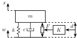
Figure 12: Relative Motion Control applied to a 1dof system
The dynamic of the system is:
\begin{equation} ms^2x = F_d - kx - csx + kw + csw + F \end{equation}In terms of the stage deformation \(d = x - w\):
\begin{equation} (ms^2 + cs + k) d = -ms^2 w + F_d + F \end{equation}The relative motion control law is:
\begin{equation} K = -g s \end{equation}Thus, the applied force is:
\begin{equation} F = -g s d \end{equation}And the new dynamics will be:
\begin{equation} d = w \frac{-ms^2}{ms^2 + (c + g)s + k} + F_d \frac{1}{ms^2 + (c + g)s + k} + F \frac{1}{ms^2 + (c + g)s + k} \end{equation}And thus damping is added.
If critical damping is wanted:
\begin{equation} \xi = \frac{1}{2}\frac{c + g}{\sqrt{km}} = \frac{1}{2} \end{equation}This corresponds to a gain:
\begin{equation} g = \sqrt{km} - c \end{equation}3.1.2 Matlab Example
Let define the system parameters.
  m = 50; % [kg]
  k = 1e6; % [N/m]
  c = 1e3; % [N/(m/s)]
The state space model of the system is defined below.
  A = [-c/m -k/m;
       1     0];

  B = [1/m 1/m -1;
       0   0    0];

  C = [ 0  1;
       -c -k];

  D = [0 0 0;
       1 0 0];

  sys = ss(A, B, C, D);
  sys.InputName = {'F', 'Fd', 'wddot'};
  sys.OutputName = {'d', 'Fm'};
  sys.StateName = {'ddot', 'd'};
The controller \(K_\text{RMC}\) is:
  Krmc = -(sqrt(k*m)-c)*s;
  Krmc.InputName = {'d'};
  Krmc.OutputName = {'F'};
And the closed loop system is computed below.
sys_rmc = feedback(sys, Krmc, 'name', +1);
3.2 Control Design
Let’s load the undamped plant:
load('./mat/active_damping_uniaxial_plants.mat', 'G');
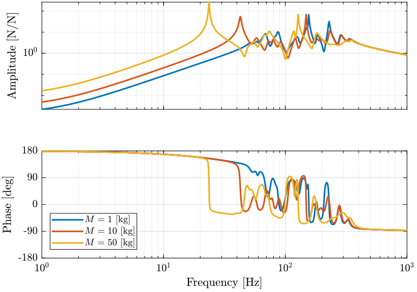
Let’s look at the transfer function from actuator forces in the nano-hexapod to the measured displacement of the actuator for all 6 pairs of actuator/sensor (figure 14).
The Relative Motion Controller is defined below. A Low pass Filter is added to make the controller transfer function proper.
K_rmc = s*50000/(1 + s/2/pi/10000);
The obtained loop gains are shown in figure 15.
3.3 Identification of the damped plant
Let’s initialize the system prior to identification.
  initializeReferences();
  initializeGround();
  initializeGranite();
  initializeTy();
  initializeRy();
  initializeRz();
  initializeMicroHexapod();
  initializeAxisc();
  initializeMirror();
  initializeNanoHexapod('actuator', 'piezo');
  initializeSample('mass', 50);
And initialize the controllers.
  K = tf(zeros(6));
  save('./mat/controllers_uniaxial.mat', 'K', '-append');
  K_iff = tf(zeros(6));
  save('./mat/controllers_uniaxial.mat', 'K_iff', '-append');
  K_rmc = -K_rmc*eye(6);
  save('./mat/controllers_uniaxial.mat', 'K_rmc', '-append');
  K_dvf = tf(zeros(6));
  save('./mat/controllers_uniaxial.mat', 'K_dvf', '-append');
We identify the system dynamics now that the RMC controller is ON.
G_rmc = identifyPlant();
And we save the damped plant for further analysis.
save('./mat/active_damping_uniaxial_plants.mat', 'G_rmc', '-append');
3.4 Sensitivity to disturbances
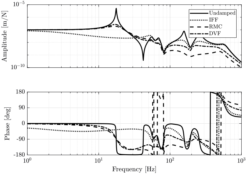
As shown in figure 16, RMC control succeed in lowering the sensitivity to disturbances near resonance of the system.
3.6 Conclusion
Relative Motion Control:
4 Direct Velocity Feedback
All the files (data and Matlab scripts) are accessible here.
In the Relative Motion Control (RMC), a feedback is applied between the measured velocity of the platform to the actuator force input.
4.1 One degree-of-freedom example
4.1.1 Equations
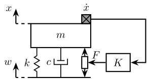
Figure 19: Direct Velocity Feedback applied to a 1dof system
The dynamic of the system is:
\begin{equation} ms^2x = F_d - kx - csx + kw + csw + F \end{equation}In terms of the stage deformation \(d = x - w\):
\begin{equation} (ms^2 + cs + k) d = -ms^2 w + F_d + F \end{equation}The direct velocity feedback law shown in figure 19 is:
\begin{equation} K = -g \end{equation}Thus, the applied force is:
\begin{equation} F = -g \dot{x} \end{equation}And the new dynamics will be:
\begin{equation} d = w \frac{-ms^2 - gs}{ms^2 + (c + g)s + k} + F_d \frac{1}{ms^2 + (c + g)s + k} + F \frac{1}{ms^2 + (c + g)s + k} \end{equation}And thus damping is added.
If critical damping is wanted:
\begin{equation} \xi = \frac{1}{2}\frac{c + g}{\sqrt{km}} = \frac{1}{2} \end{equation}This corresponds to a gain:
\begin{equation} g = \sqrt{km} - c \end{equation}4.1.2 Matlab Example
Let define the system parameters.
  m = 50; % [kg]
  k = 1e6; % [N/m]
  c = 1e3; % [N/(m/s)]
The state space model of the system is defined below.
  A = [-c/m -k/m;
       1     0];

  B = [1/m 1/m -1;
       0   0    0];

  C = [1 0;
       0 1;
       0 0];

  D = [0 0 0;
       0 0 0;
       0 0 1];

  sys = ss(A, B, C, D);
  sys.InputName = {'F', 'Fd', 'wddot'};
  sys.OutputName = {'ddot', 'd', 'wddot'};
  sys.StateName = {'ddot', 'd'};
Because we need \(\dot{x}\) for feedback, we compute it from the outputs
  G_xdot = [1, 0, 1/s;
            0, 1, 0];
  G_xdot.InputName = {'ddot', 'd', 'wddot'};
  G_xdot.OutputName = {'xdot', 'd'};
Finally, the system is described by sys as defined below.
sys = series(sys, G_xdot, [1 2 3], [1 2 3]);
The controller \(K_\text{DVF}\) is:
  Kdvf = tf(-(sqrt(k*m)-c));
  Kdvf.InputName = {'xdot'};
  Kdvf.OutputName = {'F'};
And the closed loop system is computed below.
sys_dvf = feedback(sys, Kdvf, 'name', +1);
The obtained sensitivity to disturbances is shown in figure 20.
4.2 Control Design
Let’s load the undamped plant:
load('./mat/active_damping_uniaxial_plants.mat', 'G');
Let’s look at the transfer function from actuator forces in the nano-hexapod to the measured velocity of the nano-hexapod platform in the direction of the corresponding actuator for all 6 pairs of actuator/sensor (figure 21).
The controller is defined below and the obtained loop gain is shown in figure 22.
K_dvf = tf(3e4);
4.3 Identification of the damped plant
Let’s initialize the system prior to identification.
  initializeReferences();
  initializeGround();
  initializeGranite();
  initializeTy();
  initializeRy();
  initializeRz();
  initializeMicroHexapod();
  initializeAxisc();
  initializeMirror();
  initializeNanoHexapod('actuator', 'piezo');
  initializeSample('mass', 50);
And initialize the controllers.
  K = tf(zeros(6));
  save('./mat/controllers_uniaxial.mat', 'K', '-append');
  K_iff = tf(zeros(6));
  save('./mat/controllers_uniaxial.mat', 'K_iff', '-append');
  K_rmc = tf(zeros(6));
  save('./mat/controllers_uniaxial.mat', 'K_rmc', '-append');
  K_dvf = -K_dvf*eye(6);
  save('./mat/controllers_uniaxial.mat', 'K_dvf', '-append');
We identify the system dynamics now that the RMC controller is ON.
G_dvf = identifyPlant();
And we save the damped plant for further analysis.
save('./mat/active_damping_uniaxial_plants.mat', 'G_dvf', '-append');
4.4 Sensitivity to disturbances
4.6 Conclusion
Direct Velocity Feedback:
5 Comparison
5.1 Load the plants
load('./mat/active_damping_uniaxial_plants.mat', 'G', 'G_iff', 'G_rmc', 'G_dvf');


