Control in the Frame of the Legs applied on the Simscape Model
Table of Contents
In this document, we apply some decentralized control to the NASS and see what level of performance can be obtained.
1 Decentralized Control
1.1 Control Schematic
The control architecture is shown in Figure 1.
The signals are:
- \(\bm{r}_\mathcal{X}\): wanted position of the sample with respect to the granite
- \(\bm{r}_{\mathcal{X}_n}\): wanted position of the sample with respect to the nano-hexapod
- \(\bm{r}_\mathcal{L}\): wanted length of each of the nano-hexapod’s legs
- \(\bm{\tau}\): forces applied in each actuator
- \(\bm{\mathcal{L}}\): measured displacement of each leg
- \(\bm{\mathcal{X}}\): measured position of the sample with respect to the granite
![]()
Figure 1: Decentralized control for reference tracking
1.2 Initialize the Simscape Model
We initialize all the stages with the default parameters.
initializeGround();
initializeGranite();
initializeTy();
initializeRy();
initializeRz();
initializeMicroHexapod();
initializeAxisc();
initializeMirror();
The nano-hexapod is a piezoelectric hexapod and the sample has a mass of 50kg.
initializeNanoHexapod('actuator', 'piezo');
initializeSample('mass', 1);
We set the references that corresponds to a tomography experiment.
initializeReferences('Rz_type', 'rotating', 'Rz_period', 1);
initializeDisturbances();
Open Loop.
initializeController('type', 'ref-track-L');
Kl = tf(zeros(6));
And we put some gravity.
initializeSimscapeConfiguration('gravity', true);
We log the signals.
initializeLoggingConfiguration('log', 'all');
1.3 Identification of the plant
Let’s identify the transfer function from \(\bm{\tau}\) to \(\bm{\mathcal{L}}\).
%% Name of the Simulink File
mdl = 'nass_model';

%% Input/Output definition
clear io; io_i = 1;
io(io_i) = linio([mdl, '/Controller'],                          1, 'openinput');  io_i = io_i + 1; % Actuator Inputs
io(io_i) = linio([mdl, '/Controller/Reference-Tracking-L/Sum'], 1, 'openoutput'); io_i = io_i + 1; % Leg length error

%% Run the linearization
G = linearize(mdl, io, 0);
G.InputName  = {'Fnl1', 'Fnl2', 'Fnl3', 'Fnl4', 'Fnl5', 'Fnl6'};
G.OutputName = {'El1', 'El2', 'El3', 'El4', 'El5', 'El6'};
1.4 Plant Analysis
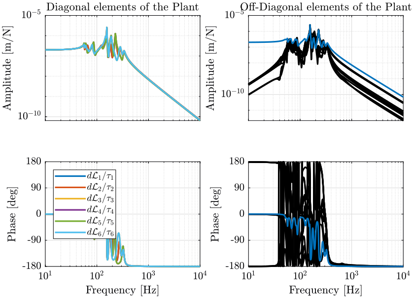
The diagonal and off-diagonal terms of the plant are shown in Figure 2.
We can see that:
- the diagonal terms have similar dynamics
- the plant is decoupled at low frequency
1.5 Controller Design
The controller consists of:
- A pure integrator
- An integrator up to little before the crossover
- A lead around the crossover
- A low pass filter with a cut-off frequency 3 times the crossover to increase the gain margin
The obtained loop gains corresponding to the diagonal elements are shown in Figure 3.
wc = 2*pi*20;
h = 1.5;

Kl = diag(1./diag(abs(freqresp(G, wc)))) * ...
     wc/s * ... % Pure Integrator
     ((s/wc*2 + 1)/(s/wc*2)) * ... % Integrator up to wc/2
     1/h * (1 + s/wc*h)/(1 + s/wc/h) * ... % Lead
     1/(1 + s/3/wc) * ... % Low pass Filter
     1/(1 + s/3/wc);

We add a minus sign to the controller as it is not included in the Simscape model.
Kl = -Kl;
1.6 Simulation
initializeController('type', 'ref-track-L');
load('mat/conf_simulink.mat');
set_param(conf_simulink, 'StopTime', '2');
sim('nass_model');
decentralized_L = simout;
save('./mat/tomo_exp_decentalized.mat', 'decentralized_L', '-append');
1.7 Results

2 HAC-LAC (IFF) Decentralized Control
We here add an Active Damping Loop (Integral Force Feedback) prior to using the Decentralized control architecture using \(\bm{\mathcal{L}}\).
2.1 Control Schematic
The control architecture is shown in Figure 1.
The signals are:
- \(\bm{r}_\mathcal{X}\): wanted position of the sample with respect to the granite
- \(\bm{r}_{\mathcal{X}_n}\): wanted position of the sample with respect to the nano-hexapod
- \(\bm{r}_\mathcal{L}\): wanted length of each of the nano-hexapod’s legs
- \(\bm{\tau}\): forces applied in each actuator
- \(\bm{\mathcal{L}}\): measured displacement of each leg
- \(\bm{\mathcal{X}}\): measured position of the sample with respect to the granite
![]()
Figure 5: Decentralized control for reference tracking
2.2 Initialize the Simscape Model
We initialize all the stages with the default parameters.
initializeGround();
initializeGranite();
initializeTy();
initializeRy();
initializeRz();
initializeMicroHexapod();
initializeAxisc();
initializeMirror();
The nano-hexapod is a piezoelectric hexapod and the sample has a mass of 50kg.
initializeNanoHexapod('actuator', 'piezo');
initializeSample('mass', 1);
We set the references that corresponds to a tomography experiment.
initializeReferences('Rz_type', 'rotating', 'Rz_period', 1);
initializeDisturbances();
Open Loop.
initializeController('type', 'ref-track-L');
Kl = tf(zeros(6));
And we put some gravity.
initializeSimscapeConfiguration('gravity', true);
We log the signals.
initializeLoggingConfiguration('log', 'all');
2.3 Initialization
initializeController('type', 'ref-track-iff-L');
K_iff = tf(zeros(6));
Kl = tf(zeros(6));
2.4 Identification for IFF
%% Name of the Simulink File
mdl = 'nass_model';

%% Input/Output definition
clear io; io_i = 1;
io(io_i) = linio([mdl, '/Controller'],                              1, 'openinput');  io_i = io_i + 1; % Actuator Inputs
io(io_i) = linio([mdl, '/Micro-Station'], 3, 'openoutput', [], 'Fnlm');  io_i = io_i + 1; % Force Sensors

%% Run the linearization
G_iff = linearize(mdl, io, 0);
G_iff.InputName  = {'Fnl1', 'Fnl2', 'Fnl3', 'Fnl4', 'Fnl5', 'Fnl6'};
G_iff.OutputName = {'Fnlm1', 'Fnlm2', 'Fnlm3', 'Fnlm4', 'Fnlm5', 'Fnlm6'};
2.5 Integral Force Feedback Controller
w0 = 2*pi*50;
K_iff = -5000/s * (s/w0)/(1 + s/w0) * eye(6);
K_iff = -K_iff;
2.6 Identification of the damped plant
%% Name of the Simulink  DehaezeFile
mdl = 'nass_model';

%% Input/Output definition
clear io; io_i = 1;
io(io_i) = linio([mdl, '/Controller'],                              1, 'input');  io_i = io_i + 1; % Actuator Inputs
io(io_i) = linio([mdl, '/Controller/Reference-Tracking-IFF-L/Sum'], 1, 'openoutput'); io_i = io_i + 1; % Leg length error

%% Run the linearization
Gd = linearize(mdl, io, 0);
Gd.InputName  = {'Fnl1', 'Fnl2', 'Fnl3', 'Fnl4', 'Fnl5', 'Fnl6'};
Gd.OutputName = {'El1', 'El2', 'El3', 'El4', 'El5', 'El6'};
2.7 Controller Design
wc = 2*pi*300;
h = 3;

Kl = diag(1./diag(abs(freqresp(Gd, wc)))) * ...
     ((s/(2*pi*20) + 1)/(s/(2*pi*20))) * ... % Pure Integrator
     ((s/(2*pi*50) + 1)/(s/(2*pi*50))) * ... % Integrator up to wc/2
     1/h * (1 + s/wc*h)/(1 + s/wc/h) * ...
     1/(1 + s/(2*wc)) * ...
     1/(1 + s/(3*wc));
isstable(feedback(Gd*Kl, eye(6), -1))
Kl = -Kl;
2.8 Simulation
initializeController('type', 'ref-track-iff-L');
load('mat/conf_simulink.mat');
set_param(conf_simulink, 'StopTime', '2');
sim('nass_model');
decentralized_iff_L = simout;
save('./mat/tomo_exp_decentalized.mat', 'decentralized_iff_L', '-append');