Simscape Uniaxial Model
Table of Contents
The idea is to use the same model as the full Simscape Model but to restrict the motion only in the vertical direction.
This is done in order to more easily study the system and evaluate control techniques.
1 Simscape Model
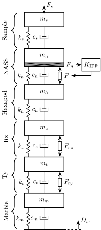
A schematic of the uniaxial model used for simulations is represented in figure 1.
The perturbations \(w\) are:
- \(F_s\): direct forces applied to the sample such as inertia forces and cable forces
- \(F_{rz}\): parasitic forces due to the rotation of the spindle
- \(F_{ty}\): parasitic forces due to scans with the translation stage
- \(D_w\): ground motion
The quantity to \(z\) to control is:
- \(D\): the position of the sample with respect to the granite
The measured quantities \(v\) are:
- \(D\): the position of the sample with respect to the granite
We study the use of an additional sensor:
- \(F_n\): a force sensor located in the nano-hexapod
- \(v_n\): an absolute velocity sensor located on the top platform of the nano-hexapod
- \(d_r\): a relative motion sensor located in the nano-hexapod
The control signal \(u\) is:
- \(F\) the force applied by the nano-hexapod actuator
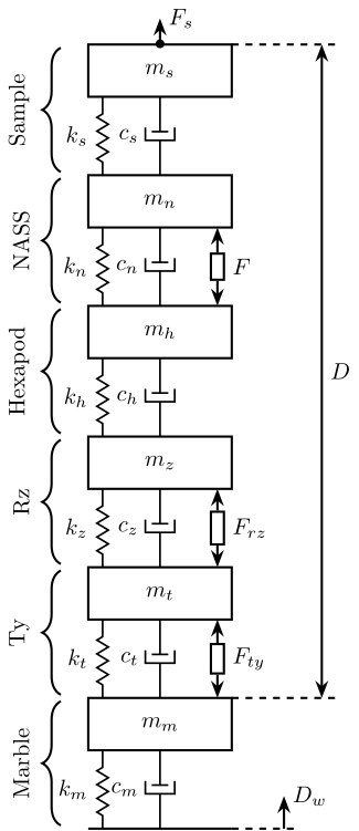
Figure 1: Schematic of the uniaxial model used
Few active damping techniques will be compared in order to decide which sensor is to be included in the system. Schematics of the active damping techniques are displayed in figure 2.
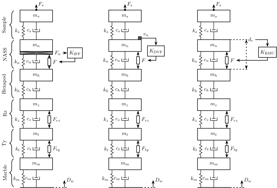
Figure 2: Comparison of used active damping techniques
2 Undamped System
2.1 Init
We initialize all the stages with the default parameters. The nano-hexapod is a piezoelectric hexapod and the sample has a mass of 50kg.
All the controllers are set to 0 (Open Loop).
2.2 Identification
We identify the dynamics of the system.
%% Options for Linearized
options = linearizeOptions;
options.SampleTime = 0;

%% Name of the Simulink File
mdl = 'sim_nano_station_uniaxial';
The inputs and outputs are defined below and corresponds to the name of simulink blocks.
%% Input/Output definition
io(1)  = linio([mdl, '/Dw'],   1, 'input'); % Ground Motion
io(2)  = linio([mdl, '/Fs'],   1, 'input'); % Force applied on the sample
io(3)  = linio([mdl, '/Fnl'],  1, 'input'); % Force applied by the NASS
io(4)  = linio([mdl, '/Fdty'], 1, 'input'); % Parasitic force Ty
io(5)  = linio([mdl, '/Fdrz'], 1, 'input'); % Parasitic force Rz

io(6)  = linio([mdl, '/Dsm'],  1, 'output'); % Displacement of the sample
io(7)  = linio([mdl, '/Fnlm'], 1, 'output'); % Force sensor in NASS's legs
io(8)  = linio([mdl, '/Dnlm'], 1, 'output'); % Displacement of NASS's legs
io(9)  = linio([mdl, '/Dgm'],  1, 'output'); % Absolute displacement of the granite
io(10) = linio([mdl, '/Vlm'],  1, 'output'); % Measured absolute velocity of the top NASS platform
Finally, we use the linearize Matlab function to extract a state space model from the simscape model.
%% Run the linearization
G = linearize(mdl, io, options);
G.InputName  = {'Dw',   ... % Ground Motion [m]
                'Fs',   ... % Force Applied on Sample [N]
                'Fn',   ... % Force applied by NASS [N]
                'Fty',  ... % Parasitic Force Ty [N]
                'Frz'};     % Parasitic Force Rz [N]
G.OutputName = {'D',    ... % Measured sample displacement x.r.t. granite [m]
                'Fnm',  ... % Force Sensor in NASS [N]
                'Dnm',  ... % Displacement Sensor in NASS [m]
                'Dgm',  ... % Asbolute displacement of Granite [m]
                'Vlm'}; ... % Absolute Velocity of NASS [m/s]
Finally, we save the identified system dynamics for further analysis.
save('./mat/uniaxial_plants.mat', 'G');
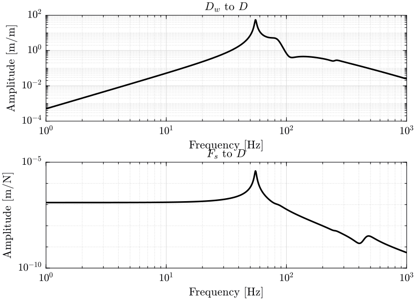
2.3 Sensitivity to Disturbances
We show several plots representing the sensitivity to disturbances:
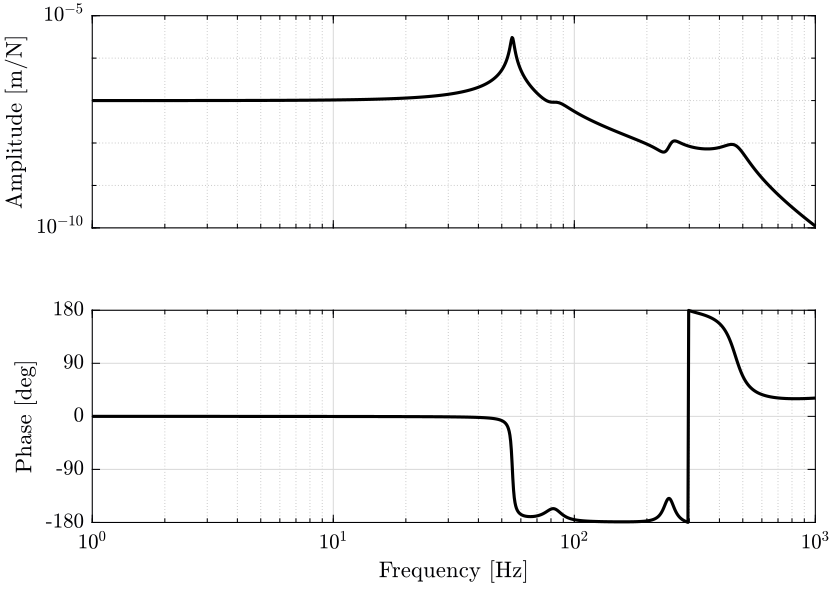
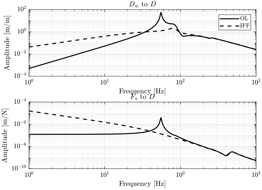
- in figure 3 the transfer functions from ground motion \(D_w\) to the sample position \(D\) and the transfer function from direct force on the sample \(F_s\) to the sample position \(D\) are shown
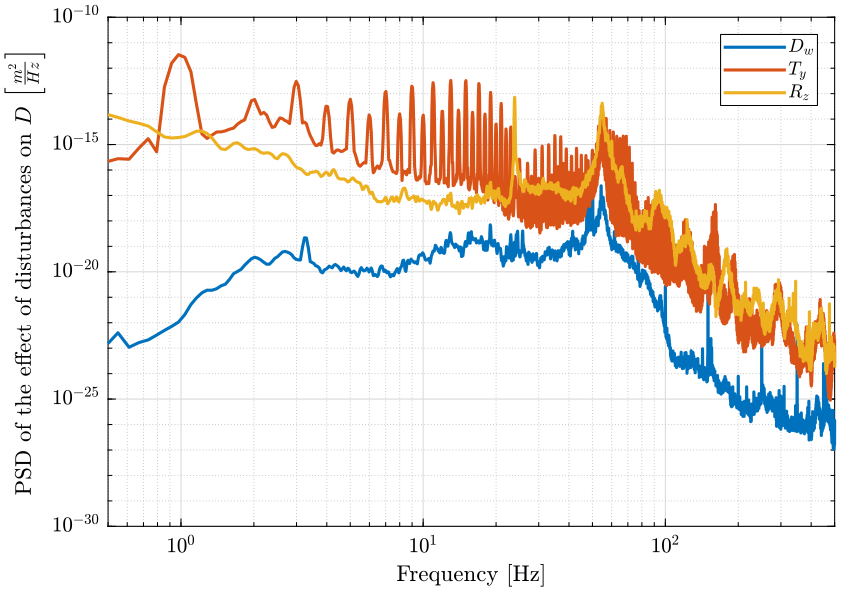
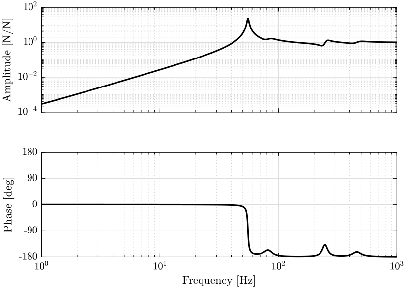
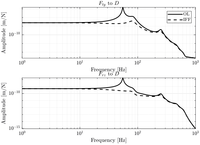
- in figure 4, it is the effect of parasitic forces of the positioning stages (\(F_{ty}\) and \(F_{rz}\)) on the position \(D\) of the sample that are shown

2.4 Noise Budget
We first load the measured PSD of the disturbance.
load('./mat/disturbances_dist_psd.mat', 'dist_f');
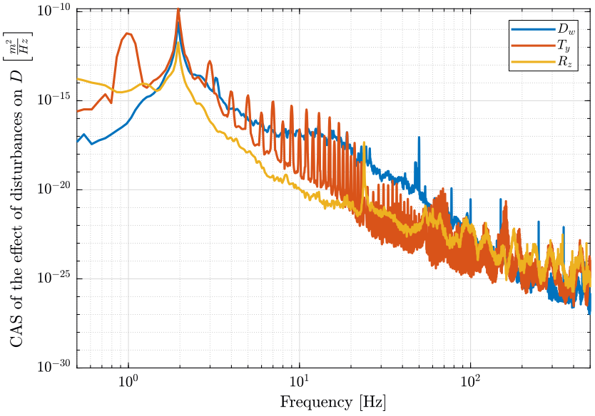
The effect of these disturbances on the distance \(D\) is computed below. The PSD of the obtain distance \(D\) due to each of the perturbation is shown in figure 5 and the Cumulative Amplitude Spectrum is shown in figure 6.
The Root Mean Square value of the obtained displacement \(D\) is computed below and can be determined from the figure 6.
3.3793e-06

3 Integral Force Feedback
3.1 Control Design
load('./mat/uniaxial_plants.mat', 'G');
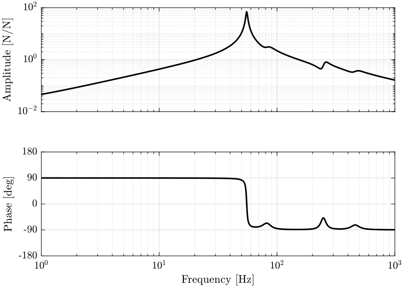
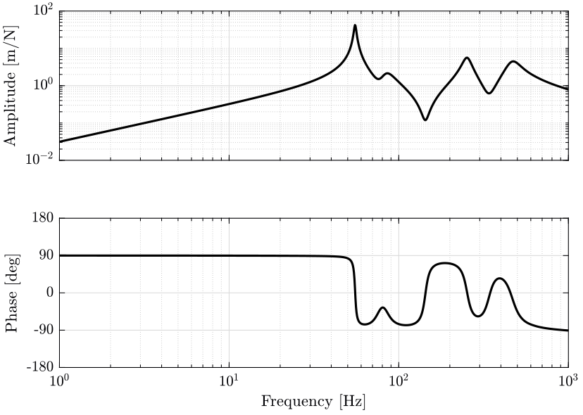
Let’s look at the transfer function from actuator forces in the nano-hexapod to the force sensor in the nano-hexapod legs for all 6 pairs of actuator/sensor.
The controller for each pair of actuator/sensor is:
K_iff = -1000/s;
3.2 Identification
Let’s initialize the system prior to identification.
initializeGround();
initializeGranite();
initializeTy();
initializeRy();
initializeRz();
initializeMicroHexapod();
initializeAxisc();
initializeMirror();
initializeNanoHexapod('actuator', 'piezo');
initializeSample('mass', 50);
All the controllers are set to 0.
K = tf(0);
save('./mat/controllers_uniaxial.mat', 'K', '-append');
K_iff = -K_iff;
save('./mat/controllers_uniaxial.mat', 'K_iff', '-append');
K_rmc = tf(0);
save('./mat/controllers_uniaxial.mat', 'K_rmc', '-append');
K_dvf = tf(0);
save('./mat/controllers_uniaxial.mat', 'K_dvf', '-append');
%% Options for Linearized
options = linearizeOptions;
options.SampleTime = 0;

%% Name of the Simulink File
mdl = 'sim_nano_station_uniaxial';
%% Input/Output definition
io(1)  = linio([mdl, '/Dw'],    1, 'input');  % Ground Motion
io(2)  = linio([mdl, '/Fs'],    1, 'input');  % Force applied on the sample
io(3)  = linio([mdl, '/Fnl'],   1, 'input');  % Force applied by the NASS
io(4)  = linio([mdl, '/Fdty'],  1, 'input');  % Parasitic force Ty
io(5)  = linio([mdl, '/Fdrz'],  1, 'input');  % Parasitic force Rz

io(6)  = linio([mdl, '/Dsm'],  1, 'output'); % Displacement of the sample
io(7)  = linio([mdl, '/Fnlm'], 1, 'output'); % Force sensor in NASS's legs
io(8)  = linio([mdl, '/Dnlm'], 1, 'output'); % Displacement of NASS's legs
io(9)  = linio([mdl, '/Dgm'],  1, 'output'); % Absolute displacement of the granite
io(10) = linio([mdl, '/Vlm'],  1, 'output'); % Measured absolute velocity of the top NASS platform
%% Run the linearization
G_iff = linearize(mdl, io, options);
G_iff.InputName  = {'Dw',   ... % Ground Motion [m]
                    'Fs',   ... % Force Applied on Sample [N]
                    'Fn',   ... % Force applied by NASS [N]
                    'Fty',  ... % Parasitic Force Ty [N]
                    'Frz'};     % Parasitic Force Rz [N]
G_iff.OutputName = {'D',    ... % Measured sample displacement x.r.t. granite [m]
                    'Fnm',  ... % Force Sensor in NASS [N]
                    'Dnm',  ... % Displacement Sensor in NASS [m]
                    'Dgm',  ... % Asbolute displacement of Granite [m]
                    'Vlm'}; ... % Absolute Velocity of NASS [m/s]
save('./mat/uniaxial_plants.mat', 'G_iff', '-append');
3.3 Sensitivity to Disturbance
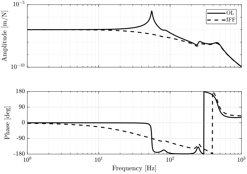
3.5 Conclusion
Integral Force Feedback:
4 Relative Motion Control
In the Relative Motion Control (RMC), a derivative feedback is applied between the measured actuator displacement to the actuator force input.
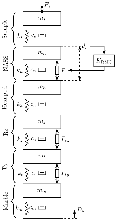
Figure 14: Uniaxial RMC Control Schematic
4.1 Control Design
load('./mat/uniaxial_plants.mat', 'G');
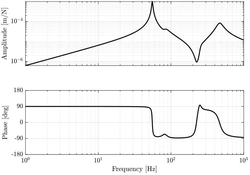
Let’s look at the transfer function from actuator forces in the nano-hexapod to the measured displacement of the actuator for all 6 pairs of actuator/sensor.

The Relative Motion Controller is defined below. A Low pass Filter is added to make the controller transfer function proper.
K_rmc = s*50000/(1 + s/2/pi/10000);
4.2 Identification
Let’s initialize the system prior to identification.
initializeGround();
initializeGranite();
initializeTy();
initializeRy();
initializeRz();
initializeMicroHexapod();
initializeAxisc();
initializeMirror();
initializeNanoHexapod('actuator', 'piezo');
initializeSample('mass', 50);
And initialize the controllers.
K = tf(0);
save('./mat/controllers_uniaxial.mat', 'K', '-append');
K_iff = tf(0);
save('./mat/controllers_uniaxial.mat', 'K_iff', '-append');
K_rmc = -K_rmc;
save('./mat/controllers_uniaxial.mat', 'K_rmc', '-append');
K_dvf = tf(0);
save('./mat/controllers_uniaxial.mat', 'K_dvf', '-append');
%% Options for Linearized
options = linearizeOptions;
options.SampleTime = 0;

%% Name of the Simulink File
mdl = 'sim_nano_station_uniaxial';
%% Input/Output definition
io(1)  = linio([mdl, '/Dw'],    1, 'input');  % Ground Motion
io(2)  = linio([mdl, '/Fs'],    1, 'input');  % Force applied on the sample
io(3)  = linio([mdl, '/Fnl'],   1, 'input');  % Force applied by the NASS
io(4)  = linio([mdl, '/Fdty'],  1, 'input');  % Parasitic force Ty
io(5)  = linio([mdl, '/Fdrz'],  1, 'input');  % Parasitic force Rz

io(6)  = linio([mdl, '/Dsm'],  1, 'output'); % Displacement of the sample
io(7)  = linio([mdl, '/Fnlm'], 1, 'output'); % Force sensor in NASS's legs
io(8)  = linio([mdl, '/Dnlm'], 1, 'output'); % Displacement of NASS's legs
io(9)  = linio([mdl, '/Dgm'],  1, 'output'); % Absolute displacement of the granite
io(10) = linio([mdl, '/Vlm'],  1, 'output'); % Measured absolute velocity of the top NASS platform
%% Run the linearization
G_rmc = linearize(mdl, io, options);
G_rmc.InputName  = {'Dw',   ... % Ground Motion [m]
                    'Fs',   ... % Force Applied on Sample [N]
                    'Fn',   ... % Force applied by NASS [N]
                    'Fty',  ... % Parasitic Force Ty [N]
                    'Frz'};     % Parasitic Force Rz [N]
G_rmc.OutputName = {'D',    ... % Measured sample displacement x.r.t. granite [m]
                    'Fnm',  ... % Force Sensor in NASS [N]
                    'Dnm',  ... % Displacement Sensor in NASS [m]
                    'Dgm',  ... % Asbolute displacement of Granite [m]
                    'Vlm'}; ... % Absolute Velocity of NASS [m/s]
save('./mat/uniaxial_plants.mat', 'G_rmc', '-append');
4.3 Sensitivity to Disturbance


4.5 Conclusion
Relative Motion Control:
5 Direct Velocity Feedback
In the Relative Motion Control (RMC), a feedback is applied between the measured velocity of the platform to the actuator force input.
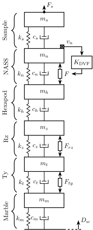
Figure 20: Uniaxial DVF Control Schematic
5.1 Control Design

5.2 Identification
Let’s initialize the system prior to identification.
initializeGround();
initializeGranite();
initializeTy();
initializeRy();
initializeRz();
initializeMicroHexapod();
initializeAxisc();
initializeMirror();
initializeNanoHexapod('actuator', 'piezo');
initializeSample('mass', 50);
And initialize the controllers.
K = tf(0);
save('./mat/controllers_uniaxial.mat', 'K', '-append');
K_iff = tf(0);
save('./mat/controllers_uniaxial.mat', 'K_iff', '-append');
K_rmc = tf(0);
save('./mat/controllers_uniaxial.mat', 'K_rmc', '-append');
K_dvf = -K_dvf;
save('./mat/controllers_uniaxial.mat', 'K_dvf', '-append');
%% Options for Linearized
options = linearizeOptions;
options.SampleTime = 0;

%% Name of the Simulink File
mdl = 'sim_nano_station_uniaxial';
%% Input/Output definition
io(1)  = linio([mdl, '/Dw'],    1, 'input');  % Ground Motion
io(2)  = linio([mdl, '/Fs'],    1, 'input');  % Force applied on the sample
io(3)  = linio([mdl, '/Fnl'],   1, 'input');  % Force applied by the NASS
io(4)  = linio([mdl, '/Fdty'],  1, 'input');  % Parasitic force Ty
io(5)  = linio([mdl, '/Fdrz'],  1, 'input');  % Parasitic force Rz

io(6)  = linio([mdl, '/Dsm'],  1, 'output'); % Displacement of the sample
io(7)  = linio([mdl, '/Fnlm'], 1, 'output'); % Force sensor in NASS's legs
io(8)  = linio([mdl, '/Dnlm'], 1, 'output'); % Displacement of NASS's legs
io(9)  = linio([mdl, '/Dgm'],  1, 'output'); % Absolute displacement of the granite
io(10) = linio([mdl, '/Vlm'],  1, 'output'); % Measured absolute velocity of the top NASS platform
%% Run the linearization
G_dvf = linearize(mdl, io, options);
G_dvf.InputName  = {'Dw',   ... % Ground Motion [m]
                    'Fs',   ... % Force Applied on Sample [N]
                    'Fn',   ... % Force applied by NASS [N]
                    'Fty',  ... % Parasitic Force Ty [N]
                    'Frz'};     % Parasitic Force Rz [N]
G_dvf.OutputName = {'D',    ... % Measured sample displacement x.r.t. granite [m]
                    'Fnm',  ... % Force Sensor in NASS [N]
                    'Dnm',  ... % Displacement Sensor in NASS [m]
                    'Dgm',  ... % Asbolute displacement of Granite [m]
                    'Vlm'}; ... % Absolute Velocity of NASS [m/s]
save('./mat/uniaxial_plants.mat', 'G_dvf', '-append');
5.3 Sensitivity to Disturbance


5.5 Conclusion
Direct Velocity Feedback:
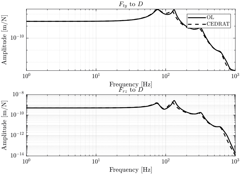
6 With Cedrat Piezo-electric Actuators
The model used for the Cedrat actuator is shown in figure 26.
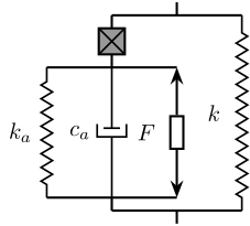
Figure 26: Schematic of the model used for the Cedrat Actuator
6.1 Identification
Let’s initialize the system prior to identification.
initializeGround();
initializeGranite();
initializeTy();
initializeRy();
initializeRz();
initializeMicroHexapod();
initializeAxisc();
initializeMirror();
initializeNanoHexapod('actuator', 'piezo');
initializeCedratPiezo();
initializeSample('mass', 50);
And initialize the controllers.
K = tf(0);
save('./mat/controllers_uniaxial.mat', 'K', '-append');
K_iff = tf(0);
save('./mat/controllers_uniaxial.mat', 'K_iff', '-append');
K_rmc = tf(0);
save('./mat/controllers_uniaxial.mat', 'K_rmc', '-append');
K_dvf = tf(0);
save('./mat/controllers_uniaxial.mat', 'K_dvf', '-append');
We identify the dynamics of the system.
%% Options for Linearized
options = linearizeOptions;
options.SampleTime = 0;

%% Name of the Simulink File
mdl = 'sim_nano_station_uniaxial_cedrat_bis';
The inputs and outputs are defined below and corresponds to the name of simulink blocks.
%% Input/Output definition
io(1)  = linio([mdl, '/Dw'],   1, 'input'); % Ground Motion
io(2)  = linio([mdl, '/Fs'],   1, 'input'); % Force applied on the sample
io(3)  = linio([mdl, '/Fnl'],  1, 'input'); % Force applied by the NASS
io(4)  = linio([mdl, '/Fdty'], 1, 'input'); % Parasitic force Ty
io(5)  = linio([mdl, '/Fdrz'], 1, 'input'); % Parasitic force Rz

io(6)  = linio([mdl, '/Dsm'],  1, 'output'); % Displacement of the sample
io(7)  = linio([mdl, '/Fnlm'], 1, 'output'); % Force sensor in NASS's legs
io(8)  = linio([mdl, '/Dnlm'], 1, 'output'); % Displacement of NASS's legs
io(9)  = linio([mdl, '/Dgm'],  1, 'output'); % Absolute displacement of the granite
io(10) = linio([mdl, '/Vlm'],  1, 'output'); % Measured absolute velocity of the top NASS platform
Finally, we use the linearize Matlab function to extract a state space model from the simscape model.
%% Run the linearization
G = linearize(mdl, io, options);
G.InputName  = {'Dw',   ... % Ground Motion [m]
                'Fs',   ... % Force Applied on Sample [N]
                'Fn',   ... % Force applied by NASS [N]
                'Fty',  ... % Parasitic Force Ty [N]
                'Frz'};     % Parasitic Force Rz [N]
G.OutputName = {'D',    ... % Measured sample displacement x.r.t. granite [m]
                'Fnm',  ... % Force Sensor in NASS [N]
                'Dnm',  ... % Displacement Sensor in NASS [m]
                'Dgm',  ... % Asbolute displacement of Granite [m]
                'Vlm'}; ... % Absolute Velocity of NASS [m/s]
6.2 Control Design
Let’s look at the transfer function from actuator forces in the nano-hexapod to the force sensor in the nano-hexapod legs for all 6 pairs of actuator/sensor.
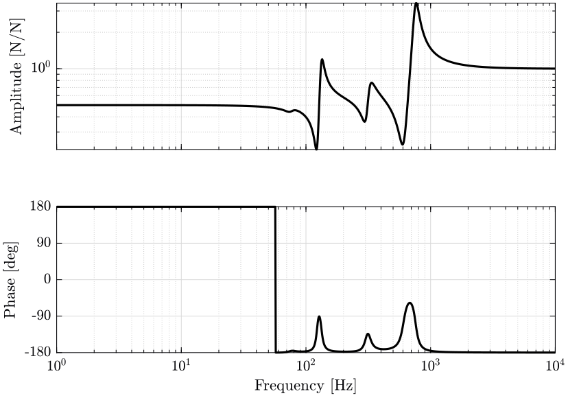
The controller for each pair of actuator/sensor is:
K_cedrat = -5000/s;

6.3 Identification
Let’s initialize the system prior to identification.
initializeGround();
initializeGranite();
initializeTy();
initializeRy();
initializeRz();
initializeMicroHexapod();
initializeAxisc();
initializeMirror();
initializeNanoHexapod('actuator', 'piezo');
initializeCedratPiezo();
initializeSample('mass', 50);
All the controllers are set to 0.
K = tf(0);
save('./mat/controllers_uniaxial.mat', 'K', '-append');
K_iff = -K_cedrat;
save('./mat/controllers_uniaxial.mat', 'K_iff', '-append');
K_rmc = tf(0);
save('./mat/controllers_uniaxial.mat', 'K_rmc', '-append');
K_dvf = tf(0);
save('./mat/controllers_uniaxial.mat', 'K_dvf', '-append');
%% Options for Linearized
options = linearizeOptions;
options.SampleTime = 0;

%% Name of the Simulink File
mdl = 'sim_nano_station_uniaxial_cedrat_bis';
%% Input/Output definition
io(1)  = linio([mdl, '/Dw'],    1, 'input');  % Ground Motion
io(2)  = linio([mdl, '/Fs'],    1, 'input');  % Force applied on the sample
io(3)  = linio([mdl, '/Fnl'],   1, 'input');  % Force applied by the NASS
io(4)  = linio([mdl, '/Fdty'],  1, 'input');  % Parasitic force Ty
io(5)  = linio([mdl, '/Fdrz'],  1, 'input');  % Parasitic force Rz

io(6)  = linio([mdl, '/Dsm'],  1, 'output'); % Displacement of the sample
io(7)  = linio([mdl, '/Fnlm'], 1, 'output'); % Force sensor in NASS's legs
io(8)  = linio([mdl, '/Dnlm'], 1, 'output'); % Displacement of NASS's legs
io(9)  = linio([mdl, '/Dgm'],  1, 'output'); % Absolute displacement of the granite
io(10) = linio([mdl, '/Vlm'],  1, 'output'); % Measured absolute velocity of the top NASS platform
%% Run the linearization
G_cedrat = linearize(mdl, io, options);
G_cedrat.InputName  = {'Dw',   ... % Ground Motion [m]
                    'Fs',   ... % Force Applied on Sample [N]
                    'Fn',   ... % Force applied by NASS [N]
                    'Fty',  ... % Parasitic Force Ty [N]
                    'Frz'};     % Parasitic Force Rz [N]
G_cedrat.OutputName = {'D',    ... % Measured sample displacement x.r.t. granite [m]
                    'Fnm',  ... % Force Sensor in NASS [N]
                    'Dnm',  ... % Displacement Sensor in NASS [m]
                    'Dgm',  ... % Asbolute displacement of Granite [m]
                    'Vlm'}; ... % Absolute Velocity of NASS [m/s]
% save('./mat/uniaxial_plants.mat', 'G_cedrat', '-append');
6.4 Sensitivity to Disturbance


6.6 Conclusion
This gives similar results than with a classical force sensor.
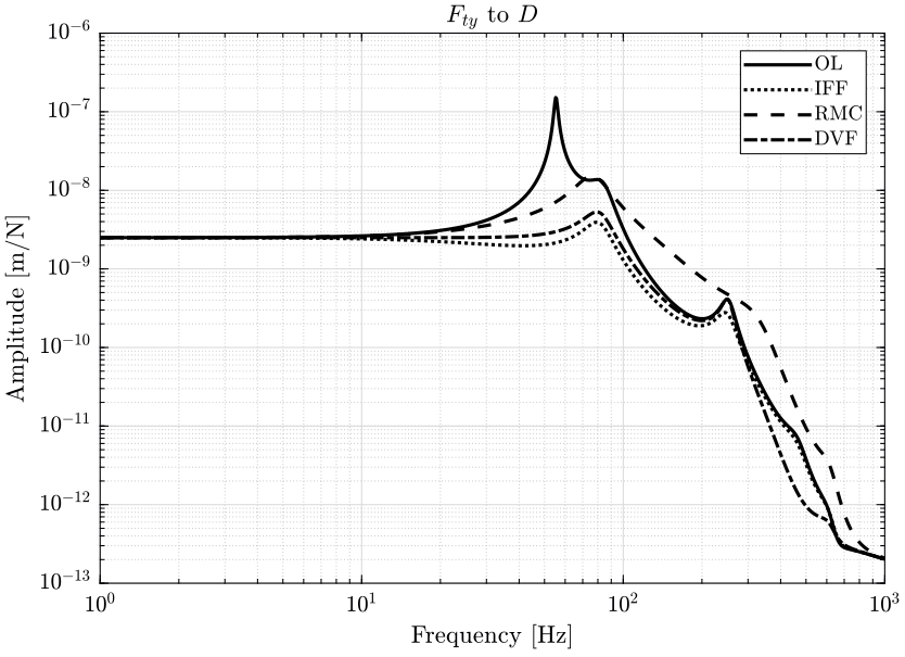
7 Comparison of Active Damping Techniques
7.1 Load the plants
load('./mat/uniaxial_plants.mat', 'G', 'G_iff', 'G_rmc', 'G_dvf');
7.2 Sensitivity to Disturbance


7.3 Noise Budget
We first load the measured PSD of the disturbance.
load('./mat/disturbances_dist_psd.mat', 'dist_f');
The effect of these disturbances on the distance \(D\) is computed for all active damping techniques. We then compute the Cumulative Amplitude Spectrum (figure 36).
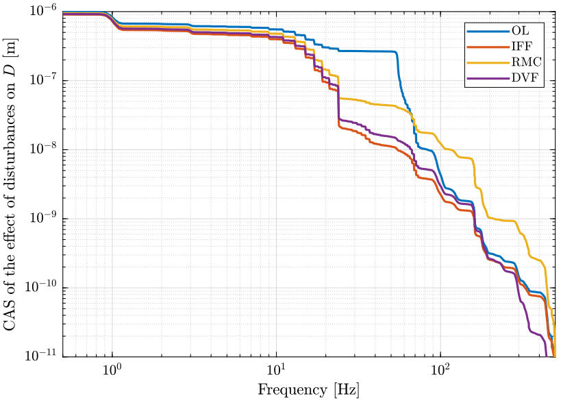
Figure 36: Comparison of the Cumulative Amplitude Spectrum of \(D\) for different active damping techniques (png, pdf)
The obtained Root Mean Square Value for each active damping technique is shown below.
| D [m rms] | |
|---|---|
| OL | 3.38e-06 |
| IFF | 3.40e-06 |
| RMC | 3.37e-06 |
| DVF | 3.38e-06 |
It is important to note that the effect of direct forces applied to the sample are not taken into account here.

7.5 Conclusion
| IFF | RMC | DVF | |
|---|---|---|---|
| Sensor Type | Force sensor | Relative Motion | Inertial |
| Guaranteed Stability | + | + | - |
| Sensitivity (\(D_w\)) | - | + | - |
| Sensitivity (\(F_s\)) | - (at low freq) | + | + |
| Sensitivity (\(F_{ty,rz}\)) | + | - | + |
| Overall RMS of \(D\) | = | = | = |
8 Voice Coil
8.1 Init
We initialize all the stages with the default parameters. The nano-hexapod is an hexapod with voice coils and the sample has a mass of 50kg.
All the controllers are set to 0 (Open Loop).
8.2 Identification
We identify the dynamics of the system.
%% Options for Linearized
options = linearizeOptions;
options.SampleTime = 0;

%% Name of the Simulink File
mdl = 'sim_nano_station_uniaxial';
The inputs and outputs are defined below and corresponds to the name of simulink blocks.
%% Input/Output definition
io(1)  = linio([mdl, '/Dw'],   1, 'input'); % Ground Motion
io(2)  = linio([mdl, '/Fs'],   1, 'input'); % Force applied on the sample
io(3)  = linio([mdl, '/Fnl'],  1, 'input'); % Force applied by the NASS
io(4)  = linio([mdl, '/Fdty'], 1, 'input'); % Parasitic force Ty
io(5)  = linio([mdl, '/Fdrz'], 1, 'input'); % Parasitic force Rz

io(6)  = linio([mdl, '/Dsm'],  1, 'output'); % Displacement of the sample
io(7)  = linio([mdl, '/Fnlm'], 1, 'output'); % Force sensor in NASS's legs
io(8)  = linio([mdl, '/Dnlm'], 1, 'output'); % Displacement of NASS's legs
io(9)  = linio([mdl, '/Dgm'],  1, 'output'); % Absolute displacement of the granite
io(10) = linio([mdl, '/Vlm'],  1, 'output'); % Measured absolute velocity of the top NASS platform
Finally, we use the linearize Matlab function to extract a state space model from the simscape model.
%% Run the linearization
G_vc = linearize(mdl, io, options);
G_vc.InputName  = {'Dw',   ... % Ground Motion [m]
                   'Fs',   ... % Force Applied on Sample [N]
                   'Fn',   ... % Force applied by NASS [N]
                   'Fty',  ... % Parasitic Force Ty [N]
                   'Frz'};     % Parasitic Force Rz [N]
G_vc.OutputName = {'D',    ... % Measured sample displacement x.r.t. granite [m]
                   'Fnm',  ... % Force Sensor in NASS [N]
                   'Dnm',  ... % Displacement Sensor in NASS [m]
                   'Dgm',  ... % Asbolute displacement of Granite [m]
                   'Vlm'}; ... % Absolute Velocity of NASS [m/s]
Finally, we save the identified system dynamics for further analysis.
save('./mat/uniaxial_plants.mat', 'G_vc', '-append');
8.3 Sensitivity to Disturbances
We load the dynamics when using a piezo-electric nano hexapod to compare the results.
load('./mat/uniaxial_plants.mat', 'G');
We show several plots representing the sensitivity to disturbances:
- in figure 38 the transfer functions from ground motion \(D_w\) to the sample position \(D\) and the transfer function from direct force on the sample \(F_s\) to the sample position \(D\) are shown
- in figure 39, it is the effect of parasitic forces of the positioning stages (\(F_{ty}\) and \(F_{rz}\)) on the position \(D\) of the sample that are shown


8.4 Noise Budget
We first load the measured PSD of the disturbance.
load('./mat/disturbances_dist_psd.mat', 'dist_f');
The effect of these disturbances on the distance \(D\) is computed below. The PSD of the obtain distance \(D\) due to each of the perturbation is shown in figure 40 and the Cumulative Amplitude Spectrum is shown in figure 41.
The Root Mean Square value of the obtained displacement \(D\) is computed below and can be determined from the figure 41.
4.8793e-06

Even though the RMS value of the displacement \(D\) is lower when using a piezo-electric actuator, the motion is mainly due to high frequency disturbances which are more difficult to control (an higher control bandwidth is required).
Thus, it may be desirable to use voice coil actuators.
8.5 Integral Force Feedback

8.6 Identification of the Damped Plant
Let’s initialize the system prior to identification.
initializeGround();
initializeGranite();
initializeTy();
initializeRy();
initializeRz();
initializeMicroHexapod();
initializeAxisc();
initializeMirror();
initializeNanoHexapod('actuator', 'lorentz');
initializeSample('mass', 50);
All the controllers are set to 0.
K = tf(0);
save('./mat/controllers_uniaxial.mat', 'K', '-append');
K_iff = -K_iff;
save('./mat/controllers_uniaxial.mat', 'K_iff', '-append');
K_rmc = tf(0);
save('./mat/controllers_uniaxial.mat', 'K_rmc', '-append');
K_dvf = tf(0);
save('./mat/controllers_uniaxial.mat', 'K_dvf', '-append');
%% Options for Linearized
options = linearizeOptions;
options.SampleTime = 0;

%% Name of the Simulink File
mdl = 'sim_nano_station_uniaxial';
%% Input/Output definition
io(1)  = linio([mdl, '/Dw'],    1, 'input');  % Ground Motion
io(2)  = linio([mdl, '/Fs'],    1, 'input');  % Force applied on the sample
io(3)  = linio([mdl, '/Fnl'],   1, 'input');  % Force applied by the NASS
io(4)  = linio([mdl, '/Fdty'],  1, 'input');  % Parasitic force Ty
io(5)  = linio([mdl, '/Fdrz'],  1, 'input');  % Parasitic force Rz

io(6)  = linio([mdl, '/Dsm'],  1, 'output'); % Displacement of the sample
io(7)  = linio([mdl, '/Fnlm'], 1, 'output'); % Force sensor in NASS's legs
io(8)  = linio([mdl, '/Dnlm'], 1, 'output'); % Displacement of NASS's legs
io(9)  = linio([mdl, '/Dgm'],  1, 'output'); % Absolute displacement of the granite
io(10) = linio([mdl, '/Vlm'],  1, 'output'); % Measured absolute velocity of the top NASS platform
%% Run the linearization
G_vc_iff = linearize(mdl, io, options);
G_vc_iff.InputName  = {'Dw',   ... % Ground Motion [m]
                       'Fs',   ... % Force Applied on Sample [N]
                       'Fn',   ... % Force applied by NASS [N]
                       'Fty',  ... % Parasitic Force Ty [N]
                       'Frz'};     % Parasitic Force Rz [N]
G_vc_iff.OutputName = {'D',    ... % Measured sample displacement x.r.t. granite [m]
                       'Fnm',  ... % Force Sensor in NASS [N]
                       'Dnm',  ... % Displacement Sensor in NASS [m]
                       'Dgm',  ... % Asbolute displacement of Granite [m]
                       'Vlm'}; ... % Absolute Velocity of NASS [m/s]
8.7 Noise Budget

8.8 Conclusion
The use of voice coil actuators would allow a better disturbance rejection for a fixed bandwidth compared with a piezo-electric hexapod.
Similarly, it would require much lower bandwidth to attain the same level of disturbance rejection for \(D\).